|
|
|
[Sponsors] | ||||
They say the only constant in life is change and that’s as true for blogs as anything else. After almost a dozen years blogging here on WordPress.com as Another Fine Mesh, it’s time to move to a new home, the … Continue reading
The post Farewell, Another Fine Mesh. Hello, Cadence CFD Blog. first appeared on Another Fine Mesh.
Welcome to the 500th edition of This Week in CFD on the Another Fine Mesh blog. Over 12 years ago we decided to start blogging to connect with CFDers across teh interwebs. “Out-teach the competition” was the mantra. Almost immediately … Continue reading
The post This Week in CFD first appeared on Another Fine Mesh.
Automated design optimization is a key technology in the pursuit of more efficient engineering design. It supports the design engineer in finding better designs faster. A computerized approach that systematically searches the design space and provides feedback on many more … Continue reading
The post Create Better Designs Faster with Data Analysis for CFD – A Webinar on March 28th first appeared on Another Fine Mesh.
It’s nice to see a healthy set of events in the CFD news this week and I’d be remiss if I didn’t encourage you to register for CadenceCONNECT CFD on 19 April. And I don’t even mention the International Meshing … Continue reading
The post This Week in CFD first appeared on Another Fine Mesh.
Some very cool applications of CFD (like the one shown here) dominate this week’s CFD news including asteroid impacts, fish, and a mesh of a mesh. For those of you with access, NAFEM’s article 100 Years of CFD is worth … Continue reading
The post This Week in CFD first appeared on Another Fine Mesh.
This week’s aggregation of CFD bookmarks from around the internet clearly exhibits the quote attributed to Mark Twain, “I didn’t have time to write a short letter, so I wrote a long one instead.” Which makes no sense in this … Continue reading
The post This Week in CFD first appeared on Another Fine Mesh.
Severe weather — like thunderstorms, tornadoes, and hurricanes — can push air upward into a higher layer of the atmosphere and trigger gravity waves. Aboard the International Space Station (ISS), the Atmospheric Waves Experiment (AWE) instrument captures these waves by looking for variations in the brightness of Earth’s airglow (above). Recently, when Hurricane Helene hit the southeastern United States, AWE caught a series of gravity waves some 55 miles up, pushed by the storm (below). It’s incredible to see these long-ranging ripples spreading far beyond the heart of the storm. (Video credits: NASA Goddard and Utah State University)
A glowing arch of red, pink, and white anchors this stunning composite astrophotograph. This is a STEVE (Strong Thermal Emission Velocity Enhancement) caused by a river of fast-moving ions high in the atmosphere. Above the STEVE’s glow, the skies are red; that’s due either to the STEVE or to the heat-related glow of a Stable Auroral Red (SAR) arc. Find even more beautiful astrophotography at the artist’s website and Instagram. (Image credit: L. Leroux-Géré; via APOD)
Though only 5 cm long, the squirting cucumber can spray its seeds up to 10 meters away. The little fruit does so through a clever combination of preparation and ballistic maneuvers. Ahead of launch, the plant actually moves water from the fruit into the stem; this reorients the cucumber so that its long axis sits close to 45 degrees. It also makes the stem thicker and stiffer.

When the burst happens, fruit spews out a jet of mucus that propels the seeds at up to 20 m/s. The initial seeds move the fastest — thanks to the fruit’s high-pressure reservoir — and fly the furthest. As the pressure drops, the jet slows and the fruit’s rotation sends the seeds higher, causing them to land closer to the original plant. With multiple fruits in different orientations, a single plant can spread its seeds in a fairly even ring around itself. (Research and image credit: F. Box et al.; via Gizmodo)
Just as rivers have tributaries that feed their flow, small glaciers can flow as tributaries into larger ones. This astronaut photo shows Siachen Glacier and four of its tributaries coming together and continuing to flow from the top to the bottom of the image. The dark parallel lines running through the glaciers are moraines, where rocks and debris are carried along by the ice. Those seen here are medial moraines left by the joining of tributaries. When glaciers retreat, moraines are often left behind, strewn with sediment that ranges from the fine powder of glacial flour all the way to enormous boulders. (Image credit: NASA; via NASA Earth Observatory)
In mid-January 2022, the Hunga Tonga-Hunga Ha’apai (HTHH) volcano had one of the most massive eruptions ever recorded, destroying an island, generating a tsunami, and blanketing Tonga in ash. Volcanologists are accustomed to monitoring nearby seismic equipment for signs of an imminent eruption, but researchers found that the HTHH eruption generated a surface-level seismic wave picked up by detectors 750 kilometers away about 15 minutes before the eruption began. They propose that the seismic wave occurred when the oceanic crust beneath the caldera fractured. That fracture could have allowed seawater and magma to mix above the volcano’s subsurface magma chamber, creating the explosive trigger for the eruption. Their finding suggests that real-time monitoring for these distant signals could provide valuable early warning of future eruptions. (Image credit: NASA Earth Observatory; research credit: T. Horiuchi et al.; via Gizmodo and AGU News)
Striped clouds appear to converge over a mountaintop in this photo, but that’s an illusion. In reality, these clouds are parallel and periodic; it’s only the camera’s wide-angle lens that makes them appear to converge.
Wave clouds like these form when air gets pushed up and over topography, triggering an up-and-down oscillation (known as an internal wave) in the atmosphere. At the peak of the wave, cool moist air condenses water vapor into droplets that form clouds. As the air bobs back down and warms, the clouds evaporate, leaving behind a series of stripes. You can learn more about the physics behind these clouds here and here. (Image credit: Y. Beletsky; via APOD)
|
Originally Posted by wyldckat

Hi sakro,
Sadly my experience in this subject is very limited, but here are a few threads that might guide you in the right direction:
Best regards and good luck! Bruno |
 <-- this dot is just a general sign for multiplication; both multiplication of scalars and scalar multiplication of vectors can be denoted by it; obviously, if I multiply vectors, I will denote them as vectors (i.e. with an arrow above), everything that doesn't have an arrow above is a scalar
 and
and  are tangent and cotangent respectively
 is logarithm with the base of 10
 is natural logarithm
 ,
,  and
and  are all the same thing
} - e^{-a_1 \cdot (\alpha_d - \alpha_{residual})})")
 is called diffusion velocity, see, e.g., general.H line 92
 is called drift velocity, see, e.g., general.H line 63
 is declared in the createFields.H file (see line 57), which is a part of interPhaseChangeFoam, and not the part of driftFluxFoam.
 dnf install -y  python3-pip m4 flex bison git git-core mercurial cmake cmake-gui openmpi openmpi-devel metis metis-devel metis64 metis64-devel
llvm llvm-devel zlib  zlib-devel  ....
{
  echo 'export PATH=/usr/local/cuda/bin:$PATH'
  echo 'module load mpi/openmpi-x86_64'
}>> ~/.bashrc
cd ~
mkdir foam && cd foam
git clone https://git.code.sf.net/p/foam-extend/foam-extend-4.1 foam-extend-4.1
{
 echo '#source ~/foam/foam-extend-4.1/etc/bashrc'
 echo "alias fe41='source ~/foam/foam-extend-4.1/etc/bashrc' "
}>> ~/.bashrc
pip install --user PyFoam
cd ~/foam/foam-extend-4.1/etc/
cp prefs.sh-EXAMPLE prefs.sh
# Specify system openmpi
# ~~~~~~~~~~~~~~~~~~~~~~
 export WM_MPLIB=SYSTEMOPENMPI
# System installed CMake
export CMAKE_SYSTEM=1
export CMAKE_DIR=/usr/bin/cmake

# System installed Python
export PYTHON_SYSTEM=1
export PYTHON_DIR=/usr/bin/python

# System installed PyFoam
export PYFOAM_SYSTEM=1

# System installed ParaView
export PARAVIEW_SYSTEM=1
export PARAVIEW_DIR=/usr/bin/paraview

# System installed bison
export BISON_SYSTEM=1
export BISON_DIR=/usr/bin/bison

# System installed flex. FLEX_DIR should point to the directory where
# $FLEX_DIR/bin/flex is located
export FLEX_SYSTEM=1
export FLEX_DIR=/usr/bin/flex  #export FLEX_DIR=/usr

# System installed m4
export M4_SYSTEM=1
export M4_DIR=/usr/bin/m4
 foam
Allwmake.firstInstall -j
Figure 1: Structured multiblock mesh for a scramjet engine.
1586 words / 8 minutes read
Over half a century has elapsed in designing a working scramjet-powered hypersonic vehicle. Considered harder than rocket engines, designing scramjets is a massive engineering challenge. However, with newer design improvisations such as airframe integration and REST design, scramjet-powered hypersonic flights are close to becoming a reality.
With China and Russia making all the buzz about making successful scramjet-powered hypersonic flights, it looks like the game is on. The West, led by NASA, started the scramjet research in the 1950s. A couple of years into the research, early scientists quickly realized the scientific difficulties of designing scramjets engines. Some say it is harder than rocketry.
This article takes you through the different aspects of scramjet technology, starting with answering the question: what is scramjet, and how is it different from jets and rockets.
What are Scramjets? And how is it different from the Jets and Rockets:

In a jet engine, the flow inside the combustion chamber is subsonic. Even if the jet is flying at supersonic speed, the intake and the compressor slow the air down to low subsonic speed. This increases the pressure and temperature. The higher the flying speed, the higher the rise in pressure and temperatures when we slow the flow down. Normally, in jets, the compressor does the job of raising the pressure and temperature. But if we are moving fast enough, the compressor can be chucked out, and so is the turbine driving it, as just slowing the flow to subsonic conditions will raise the pressure and temperature to the required levels. So, what is left behind without a compressor and turbine is the Ramjet.

A ramjet is a simple tube with an inlet to capture the air and slow it down, a combustor to inject fuel and burn it, and an exhaust nozzle to expand the combustion products to generate thrust. Ramjets can’t start from 0 speed but need about Mach 3 to get going, and they can operate up to Mach 6. Beyond that, the rise in temperature and pressure due to the ram effect is too high for proper combustion.
As a solution, what can be done is the flow can be slowed down just a little bit, thus raising pressure and temperature, but leave it largely supersonic and see if we can do combustion in it. An engine that does just that is the Scramjet – Supersonic Combustion Ramjet. Scramjets that can start operating around Mach 6 can go up to Mach 12 or 14. The upper limit is up for debate as, near the upper Mach limit, we run into the same issue of too much rise in temperature due to slow-down effects to maintain proper combustion. Additionally, near the upper limit, external drag forces become very high, and the heating problems become even more severe.

Rockets, on the other hand, don’t suck air from the atmosphere but carry their own oxygen. Because of this, they are versatile and can fly in any planetary atmosphere and empty space. At the same time, carrying oxygen makes them heavy and less fuel-efficient. So, scramjet is the most attractive option if one wants to fly at hypersonic speeds in Earth’s atmosphere.
Lastly, if one wants to compare these propulsion systems w.r.t fuel efficiency, turbojets are the most fuel-efficient system for the Mach 0 to Mach 3 range. Between Mach 3 and 6, the ramjets are the better performers, while above Mach 6, scramjets are the best. Rockets, even though can operate over all the Mach number regimes, they have the lowest fuel efficiency as they have to carry the oxidizer with them.

The first generation of scramjet engines had a pod-style design with a large axisymmetric spike for external compression. Bearing similarity to gas turbine engines, scramjet pods were designed independently of the vehicle it was meant to propel. In the end, the design was discarded as the supersonic combustion could not overcome the external drag of the spike, as it lacked the much-needed airframe integration.
Hence, from the second generation onwards, the smooth integration of the engine with the vehicle was done. The vehicle is made long and slender for low-drag purposes, and the scramjet engine, with a 2D flow path, is mounted on its belly. The engine is positioned in the shadow of the vehicle’s bow shock to ensure that the vehicle’s forebody does some part of the air compression before entering the engine. In a way, one can say the vehicle is the engine, and the engine is the vehicle in this design.
Unfortunately, even this improved airframe integration design and 2D scramjets had its pitfalls. Ground testing of these geometries revealed that 2D scramjets were not optimum for structural efficiency and overall performance. This led to the development of the current 3rd generation scramjets involving truly 3D geometries. In this design, along with integrating the scramjet into the airframe, the combustors started to have rounded or elliptical shapes.

One example of present-day 3D scramjets is the Rectangular-to-Elliptical Shape Transition or REST scramjet engines. This class of engines has a rectangular capture area that helps smooth integration with the vehicle. The rectangle cross-section gradually transitions into an elliptical cross-section as it reaches the ‘rounded’ combustor.
An elliptical shape for the combustor is preferred over a rectangular shape because it offers a reduced surface area for the same amount of airflow. This aspect of a reduced surface area significantly lowers the engine drag and cooling requirement compared to a rectangle shape. Further, the elliptical shape reduces structural weight due to the inherent strength of rounded structures. Also, the curved shape eliminates low momentum corner flows, which are observed to severely limit engine performance.

The air inside a scramjet engine passes through three distinct processes of compression, combustion, and expansion in the 3 sections: intake, combustor, and exhaust nozzle.
The Intake: The front part of the engine, the intake, does the job of capturing the air and compressing it. At station 0, the flow is undisturbed by the engine. As it moves towards station 1, the air starts to experience compression due to the flow contraction caused by the vehicle’s fore-body. Further compression is done by 3 shock waves generated in the intake. The flow passing through shock waves raises the pressure and temperature of the flow. Each shock wave aligns the flow to the walls of the intake, and by the time the flow leaves the inlet at station 2, it will be uniform and parallel to the walls of the combustor.

The Combustor: At the entrance to the combustor, between stations 2 and 3, a short duct called an isolator exists, which separates the inlet operations from the pressure rise in the combustor. At station 3, the fuel is injected and lighted. It burns in the hot air that has been compressed by the inlet.
The Nozzle: Lastly, the combustion products expand through the exhaust nozzle located between stations 4 and 10. It’s here the thrust for the vehicle gets generated.

Although functioning-wise, a scramjet engine looks simple, designing a working engine that can sustain combustion for an extended period and survive under hypersonic conditions is a daunting challenge. Several engineering difficulties exist, starting with the challenge of mixing the fuel with air and igniting it in a high-velocity flow field within less than 1 millisecond.
The second issue is the high surface heat loads generated by hypersonic flight. These can be greater than those experienced by the space shuttle on re-entry and for longer periods. The material used to build the scramjet structure needs to be lightweight and be able to withstand elevated temperatures in excess of 2000 C. Also, thermal and structural design needs to take care of thermal expansion. Materials grow as they get heated up. So, designing a structure that does not break up as its skin heats up from room temperature to 2000 C is a major engineering challenge.
Thirdly, burning fuel in a duct can sometimes lead to choking or flow blockage. So, some mechanism needs to be built to manage it. Finally, chemical reactions can freeze in the nozzle expansion, leading to incomplete combustion.
Along with these engineering challenges, there are system-level challenges. One of the major issues is scramjets don’t work below Mach 4, so there is a need for another type of propulsion system, say, a ramjet or a rocket engine, to get it up to speed. Lastly, the nature of the scramjet operation changes considerably with the Mach number. Hence, acceleration over a large Mach range will be difficult as needed to get to space.

Given their characteristics of better fuel efficiency and high manoeuvrability, scramjets are preferred over rockets for hypersonic flights in the Earth’s atmosphere. They will likely find applications in hypersonic aeroplanes or cruisers and recoverable space launchers or accelerators. Cruisers could be a vehicle that is boosted to a certain speed by a jet-ramjet combo engine and may spend most of its time at constant velocity in the upper atmosphere. On the other hand, accelerators could probably be a part of a multi-stage rocket-scramjet combo system for low-cost reusable access to space.
Scramjets have come a long way over the last 60 years. 3D scramjet idealogy has proliferated in recent times and is been widely adopted by researchers worldwide. Also, 3D scramjets like REST have opened up the available design space, allowing possibilities for newer design variants to be tested and explored. Hopefully, this will lead to better engines with improved performance and make hypersonic flights a reality in the near future.
1. “Parametric Geometry, Structured Grid Generation, and Initial Design Study for REST-Class Hypersonic Inlets“, Paul G. Ferlemann, et al., JANNAF Airbreathing Propulsion Subcommittee Meeting, La Jolla, California, 2009.
2. “Investigation of REST-class Hypersonic Inlet Designs“, Rowan J. Gollan et al., 17th AIAA International Space Planes and Hypersonic Systems and Technologies Conference, 11-14th April 2011, San Francisco, California.
3. ” “Design of three-dimensional hypersonic inlets with rectangular-to-elliptical shape transition“, Smart, M. K et al., Journal of Propulsion and Power, Vol. 15, No. 3, 1999, pp. 408–416.
4. “Free-jet Testing of a REST Scramjet at Off-Design Conditions“, Michael K Smart et al., Smart, Michael K, et al., 25th AIAA Aerodynamic Measurement Technology and Ground Testing Conference, 5-8 June 2006, San Francisco, California.
5. “Scramjet Inlets“, Professor Michael K. Smart, RTO-EN-AVT-185.
6. “Hypersonic Airbreathing Propulsion“, David M. Van Wie, et al., Johns Hopkins APL Technical Digest, Volume 26, Number 4 (2005).
7. “Hypersonic Speed Through Scramjet Technology“, Kevin Dirscherl et al., University of Colorado at Boulder, Boulder, Colorado 80302, December 17, 2015.
By subscribing, you'll receive every new post in your inbox. Awesome!
The post Hypersonic Flights by Scramjet Engines appeared first on GridPro Blog.
Figure 1: Hexahedral mesh for accurate capturing of leakage gaps in screw compressors.
1106 words / 6 minutes read
Leakage flows stand out as the primary factor leading to decreased efficiency within screw compressors. Precisely capturing these leakage flows using enhanced grids plays a crucial role in achieving precise CFD predictions of their behavior and their consequential impact on the overall performance of the screw compressor.
Rotating volumetric machines like screw compressors or tooth compressors are used extensively in many industrial applications. It is reported that nearly 15 percent of all-electric energy produced is used for powering compressors. Even a small improvement in the efficiency of these rotary compressors will result in a significant reduction in energy consumption. In fact, a small variation in rotor shape hardly visible to the naked eye can cause a notable change in efficiency.
Research indicates that the primary factor leading to efficiency reductions in screw compressors is leakage. This leakage occurs as a result of gaps present between rotors and between rotors and the casing. Among various thermo-fluid behaviours, internal leakage has a more substantial impact, particularly when operating at lower speeds and higher pressure ratios.
With improvement in energy efficiency becoming the main objective of design and development teams, there is a growing interest in flow patterns within screw compressors, particularly focusing on the phenomenon of leakage flows.
Screw compressors operate by altering the volume of the compression chamber, leading to corresponding variations in internal pressure and temperature. As pressure builds up during compression, the compressed gas seeks to move into lower-pressure chambers through the leakage gaps.
Unfortunately, due to the helical nature of the compression process in positive displacement machines, it is very difficult to visually appreciate this leakage flow by any experimental methods. Also, the complex flows in screw compressors demand more detailed studies, which makes conducting physical experimentation very expensive. Hence, experimental studies in these machines have become less attractive, while CFD, with accurate prediction abilities along with detailed 3D flow measurement and visualization capabilities, has been accepted as the workable alternative.
In positive displacement machines, leakage flow is an inescapable devil. Due to the nature of the mating parts and the need for clearances between them, the compressor is bound to have several leakage paths. About 6 different leakage paths have been identified, as shown in Figure 2.

Out of these, only the cusp blow holes have a constant geometry, while the rest of the paths have a geometry and flow resistance that varies periodically in a way unique to each individual path. Further, the pressure difference driving the fluid along a leakage path also varies periodically in a manner that is unique to each leakage path.
Leakages can broadly be categorized into two groups. In the first kind, the leakage happens from the enclosed cavity or discharge chamber to the suction chamber. This causes a reduction in both volumetric and indicated efficiencies. While in the second group, leakage flow occurs from the enclosed cavity or the discharge chamber to the following enclosed cavity. Although the indicated efficiency reduces in this mode, the volumetric efficiency does not.

Each leakage path uniquely influences the performance of the compressor. Hence, it is important to understand the attributes of the leakage through each leakage path and the percentage by which it can impact the machine’s efficiency. This is essential because it helps prioritise the design procedures in general and specifically enhancing the rotor lobe profile.

The critical factor which affects the CFD performance prediction of twin screw compressors is the accuracy with which leakage gaps are captured by gridding strategies. Since the working chamber of a screw machine is transient in nature, we need a grid that could accurately represent the domain deformation.
One approach is simply increasing the grid points on the rotor profile. Studies have shown that grid refinement in the circumferential direction directly influences mass flow rate prediction. In contrast, it has a lesser influence on predicting pressure and power. However, since we want to do a transient simulation in a deforming domain, this gridding approach will cause quicker deterioration in grid quality and a rapid rise in computational time.

Alternatively, another effective way to tackle this discretization challenge is to locally refine only the interlobe space region. This particular area holds utmost significance in managing leakage flows. By confining the increase in cell count to the interlobe gaps and blow-hole areas, the overall grid dimensions can be maintained under control.
The benefits of mesh refinement in the vicinity of interlobe gap and blow-hole area can be seen in improved accuracy in predicting mass flow rate and leakage flows. Interlobe refinement improves the curvature capturing of rotor profiles and also the mesh quality. This is reflected in the CFD predictions.

The difference between experimental indicated power and CFD predictions on the base grid is about 2.7% at 6000 rpm and 6.6% at 8000 rpm. With interlobe grid refinement, the difference reduces to 1.4% at 6000 rpm and 2.8% at 8000 rpm.
The enhancement of the interlobe grid refinement significantly impacts the flow rate. The contrast between experimental outcomes and CFD projections on the base grid is noticeable, registering at 11% and 8.7% for 6000 rpm and 8000 rpm respectively. These disparities decrease notably to approximately 5.5% and 2.9% following grid refinement.
The volumetric efficiency prediction on the base grid is 7% lower than the experiment. With refinement, the difference reduces to 3%. As with other variables, the difference is smaller at 8000 rpm than at 6000 rpm.

Specific indicated power, reliant on indicated power and mass flow rate, displays sensitivity. At 6000 rpm, the difference between the base grid CFD prediction and experimental-specific indicated power is about 0.2 kW/m3/min, which reduces to 0.15 kW/m3/min with refinement. At 8000 rpm, the CFD predictions match with the experiment, as can be seen in Figure 7.
The findings suggest that employing finer grids leads to better capturing of the rotor geometry, thereby enhancing the accuracy of leakage loss representation. With successively refined grids, the reduction in leakage losses becomes apparent. As a result, the CFD predictions gradually align more closely with experimental data.
1. Challenges in Meshing Scroll Compressors
2. Automation of Hexahedral Meshing for Scroll Compressors
3. The Art and Science of Meshing Turbine Blades
1.“The Analysis of Leakage in a Twin Screw Compressor and its Application to Performance Improvement”, John Fleming et al., Proc Instn Mcch Engrs Vol 209, 1995.
2. “Analytical Grid Generation for accurate representation of clearances in CFD for Screw Machines”, S Rane et al., Article in British Food Journal · August 2015.
3. “Grid Generation and CFD Analysis of Variable Geometry Screw Machines”, Sham Ramchandra Rane, PhD Thesis, City University London School of Mathematics, Computer Science and Engineering August 2015.
4. “ CFD Simulations of Single- and Twin-Screw Machines with OpenFOAM”, Nicola Casari et al., Designs 2020.
5. “Numerical Modelling and Experimental Validation of Twin-Screw Expanders” Kisorthman Vimalakanthan et al., Energies 2020, 13, 4700.
6. “New insights in twin screw expander performance for small scale ORC systems from 3D CFD Analysis”, Iva Papes et al., Journal of Applied Thermal Engineering, July 15, 2015.
7. “A GRID GENERATOR FOR FLOW CALCULATIONS IN ROTARY VOLUMETRIC COMPRESSORS”, John Vande Voorde et al., European Congress on Computational Methods in Applied Sciences and Engineering, ECCOMAS 2004.
8. “CFD SIMULATION OF A TWIN SCREW EXPANDER INCLUDING LEAKAGE FLOWS”, Rainer ANDRES et al., 23rd International Compressor Engineering Conference at Purdue, July 11-14, 2016.
9. “Calculation of clearances in twin screw compressors”, Ermin Husak et al., International Conference on Compressors and their Systems 2019.
By subscribing, you'll receive every new post in your inbox. Awesome!
The post Accurate Capturing of Leakage Gaps in Screw Compressors with Hex Grids appeared first on GridPro Blog.
Figure 1: Automated gerotor pump meshing with GridPro’s structured multiblock grid generator.
1454 words / 7 minutes read
Automated hexahedral mesher empowers engineers to effortlessly scrutinize the flow behaviour, vividly understand the change in flow with the change in clearance gap, and explicitly bring out the differences in the gerotor design variant’s performances.
The unique characteristics of gerotor pumps have made them a widely used pumping device in various industries. They are compact, reliable, and inexpensive, making them a cost-effective option for fluid transfer applications. Additionally, they offer high tolerance to fluid contamination, aeration, and cavitation. By providing excellent flow control, minimal flow pulsation and low noise, they have a strong footprint in the aerospace, automotive and manufacturing sectors.
The aerospace industry uses them for cooling, lubrication, and fuel boost and transfer processes. In manufacturing, they are used for dosing, filling, dispensing, and coating applications. Gerotor pumps are also extensively used in the automotive, agriculture, and construction fields, particularly for low-pressure applications. With the progress of technology, gerotor pumps are finding new applications in the life science, industrial, and mechanical engineering sectors.
This expansion in applicability across various industries is driving the gerotor pump research for further improvement. Also, the growing environmental concern in various industries is creating a need for newer applications, which demand pumps that can improve their efficiency. Gerotor pumps, with their simple design, have presented themselves as an attractive option for these newer applications. However, the increasing demand for pumps that meet stringent specifications and shorter design cycles necessitates a cost-effective design process that can lead to optimal performance and efficiency.
This has driven further research on gerotor pumps, focusing on improving design through numerical simulation, allowing designers to identify potential performance issues and optimize their designs before building physical prototypes. By leveraging this approach, researchers are leading the way towards more efficient and reliable gerotor pump designs that meet the growing demand for pump applications in various industries.

CFD is an essential tool for the design and optimization of gerotor pumps. CFD simulations accurately predict the effect of cavitation and fluid-body interaction on performance by providing a detailed description of the fluid’s behaviour inside the pump. Due to its accuracy, CFD is often used as a benchmark for pump experiments when no experimental comparison data is available.
However, there are certain challenges in using CFD for gerotor pump design. The CFD process requires large simulation time and memory requirements, and there is a need to re-mesh the entire domain at each angular step. Further, meshing the inter-teeth clearance and constantly changing fluid domain could be a challenging task.
These constraints can delay the design verification stage, making the process time-consuming. The design engineer must mesh the volume chambers each time the design changes and perform a time-consuming simulation. In most cases, the simulation of a geometric configuration takes up to a day to generate results. This workflow hinders the effectiveness of rapid design methodologies or the easy testing of a large number of geometric configurations of the pump in a reasonable time.
The primary focus of research w.r.t meshing positive displacement machines is the development of methodologies to support rapid simulation of any geometry. Efforts are made to develop meshing methods to automatically generate high-resolution grids with optimal cell size and high quality without human intervention.
However, gerotor pump meshing is challenging due to the rotating and deforming fluid volumes created during their working cycle. The rapid transformation of the deforming fluid zone from a large pocket region to a narrow passage makes meshing extremely difficult, w.r.t maintaining cell resolution, cell quality and mesh size. Trying to attain one of these meshing objectives results in the failure of the other. On top of this, coming up with a meshing procedure to avoid human intervention further ups the difficulty levels.
Additionally, the tight clearance space, which plays a significant role in determining volumetric efficiency, presents another obstacle for CFD simulations. These clearances are extremely small, often in the range of a few microns, and impact various aspects of the pump’s performance, such as flow leakage, flow ripple, cavitation, pressure lock, torque, and power. Out of these, the flow ripple parameter is significantly affected by the design of the tip and side gaps. A high ripple in the outlet flow can cause high levels of vibration and noise in the pump.
Hence it is critically important to accurately represent these narrow gaps with high-resolution, high-quality meshes to bring out their effects in high clarity. Low-resolution coarse grids will decrease the accuracy and may lead to over or underestimation of the flow variables. Maintaining a certain mesh quality is also important, as it enables CFD to easily analyse variations in clearances and other tendencies.

Various meshing techniques have been employed over time to discretize the gerotor fluid space. Among them, overlapping meshing methods, deform and remesh methods and customised structured meshing are the most popular ones.
Overlapping meshing methods, including the overset and immersed boundary methods, are frequently used. Although they are quick to generate, they often fall short of properly resolving the boundary layer and narrow clearance gaps while also employing an excessive number of cells.
The deform and remesh method is another popular approach that offers automation but often generates grids with a large cell count. Unfortunately, these methods can cause interpolation errors and stability issues while running the CFD solvers.
While manual customised grid generation methods provide the best mesh in terms of cell quality and grid size, they demand excessive time and human effort to generate the mesh. Unlike the generic moving mesh methods, such as the immersed boundary method, manual gridding approaches, such as the structured moving/sliding methods, accurately represent the dynamic gaps.
In the structured moving/sliding mesh approach, the fluid volume of the rotor chamber is isolated from the stationary fluid volumes related to the suction and delivery port. The rotor volume is topologically similar to a ring, making it easy to create an initial structured mesh for this shape. This zone being an extrudable domain, a 2D grid is created, which is later extruded to get a 3D mesh.
The stationary fluid volumes of the suction and delivery port are meshed using unstructured approaches. They are linked to the rotor mesh volume via non-conformal interfaces.
When the inner gear surface shifts to a new position, the mesh on the surface does not simply move with it. Instead, the mesh “slides” on the inner gear surface while adjusting to conform to the new clearance between the inner and outer gear surfaces. Simultaneously, the interface connections between the rotor volume and other fluid volumes are updated. These meshing steps ensure good resolution of the clearance space while maintaining good cell quality.

GridPro addresses the gerotor pump meshing challenge with its unique single-topology multi-configuration approach. To start with, for a given instance of the inner and the outer gear position, a 2D wireframe topology is built. Since the meshing zone is 2.5D in nature, a grid in 2D is good enough, which is later extruded in the perpendicular direction to get the 3D grid. The 2D topology acts as a template, to be later used repeatedly to generate mesh for all instances of the inner and outer gear positioning.
An automated python script ensures the grids for all angular steps are generated in an automated, hands-free environment. The script rotates the inner and outer gear at a user-specified angular step of 0.1 degrees and gives out a grid with consistent mesh quality. Since the topology is the same, the mesh generated for each angular step is practically the same. This particular aspect brings in significant positive benefits when compared to an unstructured re-meshing approach where the cell count and connectivity are completely different from one angular step grid to another.
This consistency in grids generated for all instances of the gear position aids in generating superior flow field simulation results. The automated meshing environment saves time and human effort and provides the much-needed trust of the design engineer in the simulated CFD data.
Engineers can enhance their workflow for 3D CFD analyses of gerotor pumps with an automated hexahedral mesher. It will empower engineers to effortlessly scrutinize the flow behaviour inside the working chambers, vividly understand the change in flow physics with variation in clearance gap, and explicitly bring out the differences in parametric design variant’s performances.
More importantly, an automated mesher brings the engineers’ focus back to the design aspects of the pump rather than on the meshing.
By subscribing, you'll receive every new post in your inbox. Awesome!
The post Automated Hexahedral Meshing of Gerotor Pumps appeared first on GridPro Blog.
Figure 1: Block Adapted Shock Fitted Structured Grid for Hypersonic Simulations for Orion Reentry Capsule Configuration.
1483 words / 7 minutes read
Discover the advancements in flow feature-aligned structured grid generation for hypersonic simulations with strong shocks. This article explores the innovative shock-fitting feature in GridPro, which aligns mesh blocks with shock contours to improve accuracy and reduce computational costs. Learn how this new technique outperforms traditional methods by simplifying grid alignment and enhancing shock capture, making it ideal for complex geometries with multiple shocks.
Computational fluid dynamics is critically essential and highly recommended for predicting the aerothermal environment of reentry vehicles experiencing hypersonic flow. In these regimes, shock waves are a dominant flow phenomenon. It is needless to say capturing these shock waves to the finest level possible is critically essential for accurately predicting the hypersonic flow field. Traditionally, two distinct approaches, known as shock fitting and shock capturing, have been widely used to handle such discontinuities.
Shock Capturing involves implicit handling of shocks through numerical schemes that can deal with discontinuities without explicitly locating them. They employ artificial viscosity or flux limiters to stabilize the solution and prevent non-physical oscillations. However, they may produce smeared shock profiles and require fine grids to achieve higher accuracy, potentially increasing computational costs.
Shock Fitting, on the other hand, explicitly tracks the position of shock waves within the CFD domain. It treats the shock as a moving boundary within the domain, solving additional equations to update its position and speed. This approach provides a sharp and accurate representation of shocks without the smearing effects seen in shock capturing. However, it is more complex to implement, requiring additional equations for shock dynamics and frequent grid adjustments to accommodate moving shocks.
To sum up, shock capturing is robust, versatile and easier to apply to a wide range of problems, albeit with potential accuracy trade-offs. while on the other hand, shock fitting offers superior accuracy for specific applications but at the cost of increased complexity and implementation effort.
To tackle the challenge of accurately representing shock features, engineers at GridPro have developed a new feature, which enables shock-fitted structured grid generation by aligning grid blocks with the shock contour. This article provides an in-depth discussion of this novel method.
The computational fluid dynamics workflow begins with the creation of a base structured multi-block mesh for the desired geometry and conducting an initial CFD simulation using this mesh. Following this, post-processing is carried out to extract an iso-contour Mach sheet that passes through the shock.
This Mach iso-contour surface serves as a reference to realign the mesh blocks. By adjusting the topology to align the blocks with the shock, a new mesh is generated with cells more effectively positioned to capture the thin, three-dimensional shock. This updated grid is then used for a second simulation, and the process is repeated until the user achieves the desired level of accuracy in the results.

To commence the simulation, an initial structured grid must be created. The baseline mesh adopts an analytical sphere as its outer domain, with no specialized adjustments made to accommodate shock features. This streamlined approach allows for swift setup of the initial grid, requiring minimal effort and time investment. Furthermore, maintaining symmetry along the X-Y plane aids in reducing grid points, thereby enhancing simulation efficiency.


Following the structured grid generation, the flow simulation is conducted using MISTRAL, a Navier-Stokes solver tailored for reacting flows.
Initially, the solution is computed on an Euler grid, without implementing specialized boundary layer clustering for the capsule wall.
This simplification is deliberate, aimed at minimizing computational time, as the primary focus of the initial iteration is the extraction of the shock surface.
The process of detecting and extracting shocks commences with the post-processing of the MISTRAL solution to derive the Mach distribution in the flow domain. The location of the bow shock is determined by selecting a percentage of the freestream Mach number, typically ranging between 90% to 95%. Subsequently, a Mach iso-contour sheet is extracted from the flow solution utilizing the Paraview visualization package. Following the extraction, the Mach sheet is saved as an STL file and imported into GridPro for further processing.

Given the coarse resolution of the bow shock on the initial grid, the Mach iso-surface may display roughness. To address this, a smoothing process becomes imperative. Utilizing GridPro’s built-in subdivision scheme, the extracted Mach contour is smoothed and enhanced to make it more suitable for subsequent stages of the shock-capturing procedure.

With the shock contour sheet in hand, we’re ready to delve into the actual shock-capturing process. Firstly, the tool automatically pinpoints the block faces closest to the extracted shock contour sheet. Next, those faces proximate to the shock undergo splitting and a buffer layer of the block is created around the shock. Notably, this splitting operation maintains the integrity of the block structure, relieving the user from the burden of resolving any ensuing issues.
Following this, blocks lying beyond the buffer layer are automatically deleted (as shown in Figure 7a). Next, a new outer domain surface, encapsulating the capsule is generated by scaling up the shock contour sheet by a small percentage.

Consequently, the outer faces of the buffer layer blocks serve as the boundary faces of this new outer envelope, establishing a zone characterized by shock-aligned grid lines. A detailed view of the mesh obtained after the initial shock-fitting iteration is presented in Figure 7b.
It’s important to note that the decision to split the topology hinges on the specifics of each case. In scenarios where there’s no need to reduce the computational domain’s size, this step may be bypassed. However, in instances like the one described here, where pinpointing the shock’s location and the primary flow physics region is challenging before simulation, employing this process can significantly slash the computational domain by over half. Such reduction translates into substantial savings in computational time and resources.
The Mach contour image in Figure 8 clearly demonstrates that the shock is significantly crisper and closer to the body. The cells are noticeably better aligned with both the general flow direction and the shock’s location. Remarkably, just one shock-fitting iteration was sufficient to achieve a good solution, highlighting the efficiency and effectiveness of the block-adapted shock alignment method.

The computed results are compared to data from Reference, which utilizes the US3D code. Figure 9 compares surface pressure variation along the symmetry line (in the z direction) of the capsule. The maximum pressure error is less than 1%, which is well within acceptable standards, validating the quality of the obtained solution.

The next test case considered to validate the tool was the leading nose region of the Space Launch System. Two structured grids were generated- a baseline grid (0.7 million) and a shock-fitted grid (0.762 million) and CFD computations were done at Mach 5. Figure 10 shows the grids and the improvement in the flow field with the block-adapted shock alignment method.

The third test case involves hypersonic simulations for a blunt body configuration at Mach 20. Here also 2 grids – Baseline (5.92 million) and shock-fitted grids (5.61 million) were employed. Figure 11 below shows the crisp representation of the bow shock with block-adapted shock-fitted grids.

The block-adapted shock alignment approach is straightforward to implement, requiring fewer re-meshing and CFD simulation iterations compared to other shock-fitting procedures or adaptive shock-capturing methods. Additionally, it only increases the cell count of the base grid by a smaller amount.
This method can be seamlessly integrated into the existing GridPro-CFD solver-post-processor loop without any modifications. The base-structured hexahedral meshes, with their inherently low dissipation properties, enhance shock capture accuracy. By using the shock surface to identify shock-interfering blocks and refining these blocks through wrapping, the resulting grid is sufficiently dense and aligned with the shock contour to capture it accurately. Typically, executing this loop for one or two iterations is sufficient.
A key advantage of this approach is the minimal increase in cell count and the presence of one-to-one connected cells. Due to the limited number of iterative loops and uni-directional cell refinement, the increase in cell count remains marginal. Importantly, any computational fluid dynamics solver compatible with hexahedral meshes can utilize the shock-fitted grids, as one-to-one cell connectivity with neighbouring cells is consistently maintained.
A workflow for shock-fitting grid generation has been developed and rigorously tested, proving effective in accurately capturing shocks. Demonstrated through the Orion re-entry capsule and SLS rocket test cases, this new mesh generation process can rapidly produce accurate CFD estimates for hypersonic geometries. It stands as a viable and promising alternative to traditional shock-fitting or shock-capturing mesh generation methods. The efficacy of these novel approaches is evident, showcasing significant improvements in the flow field due to the highly precise representation of the shock contour.
By subscribing, you'll receive every new post in your inbox. Awesome!
The post Fast and Accurate Hypersonic CFD Simulations: Impact of Automatic Shock-Aligned Meshes appeared first on GridPro Blog.
Figure 1: GridPro Version 9 Feature Image.
1532 words / 7 minutes read
In the ever-evolving landscape of grid generation, the goal of having an autonomous and reliable CFD simulation is the driving force behind progress. We’re thrilled to announce the release of GridPro Version 9, a major update that brings many new features, improvements, and powerful tools to empower users to achieve this vision. This release marks a significant milestone in our commitment to automate structured meshing. We have two new verticals released along with GridPro Version 9:
This article presents a few highlights. To learn more about other features packed in Version 9, Check out the release notes and What’s New.
To align ourselves with CFD_Vision_2030_Roadmap, we now use ESP as our modelling environment. With the introduction of this new environment, we aim to provide an adequate linkage between GridPro and the upfront CAD system. We have implemented a host of CAD creation tools, which enables users to create basic geometries in GridPro using the CAD panel.
As the first linking step in any Upfront CAD package, GridPro can import the labelling and grouping from any CAD package upstream through our improved STEP file format. The labels created in CAD software can be edited or inherited as surface and boundary labels in the mesh exported from GridPro, creating a seamless integration with the solver downstream.
In GridPro Version 9, labelling/grouping can also be used to split the underlying surface mesh. In the previous version, surfaces were split to improve the volume mesh quality based on the feature angles, but now users can also split surfaces by utilizing surface labels/groups. This saves time and reduces the manual effort required to select multiple surfaces for splitting purposes.
One of the significant challenges with traditional structured meshing is to dynamically update 3D blocking in the design and analysis of many engineering applications. Especially in scenarios involving shape optimization, moving boundary problems, etc. This requires the user to regenerate the blocks for every design change. It is a tedious and very time-consuming task to recreate a block structure after every design iteration.
GridPro, being a topology-based mesher, could readily accommodate geometry variations without any additional changes to the blocking. However, when geometries have non-uniform scaling, the parts of the block topology have to be moved close to the geometry to be mapped. This could become a time-consuming process, but with the introduction of the Block Mapping tool, the mapping can be done with a few clicks.

GridPro’s flexible topology paradigm enables users to create blocks without any restrictions. This sometimes results in the user creating poorly shaped blocks. Though the mesh generation engine smooths the poorly shaped blocks, it increases the mesh convergence time. With the new topology, smoother, irregularly placed blocking is now repositioned to provide a better intuition and speed up the meshing time. With this new feature, the time for grid generation is significantly reduced by an order of magnitude in many cases.
To improve hypersonic simulation workflows, GridPro introduces a Shock Alignment feature. This innovation adapts the grid blocks to the shock formed in a baseline solution. By splitting blocks in the shock region and aligning the grid normal to the shock surface, the algorithm enhances simulation accuracy and accelerates convergence. This advancement allows users to achieve faster and more precise results, optimizing their computational fluid dynamics analyses. With GridPro’s Shock Alignment, engineers and researchers can tackle complex hypersonic flows more efficiently and reliably. (Check out the paper published in the AIAA Hypersonics Conference: A Shock Fitting Technique For Hypersonic Flows Using Hexahedral Meshes.)

In GridPro, we have combined the benefits of unstructured meshing like local refinement, mesh adaptation, and multi-scale meshing by adapting the multi-block structure. This is done with a feature called Nesting, In this version we have released another flavour of nesting called the clamped nest. Clamped nesting aggressively refines the mesh near the geometry while coarsening it outside the region. This technique is particularly effective in creating highly refined regions, especially for LES and DNS simulations.

To speed up the block creation time for repeated geometries, an Array-block replication option is introduced. This provides the capability to replicate a topology in multiple directions. This tool is particularly advantageous when dealing with similar geometric patterns or shapes. Instead of creating the topology individually for each pattern, users can generate one pattern and seamlessly replicate it across self-similar geometric patterns in three different directions. Utilizing the Array feature, users can create blocking for a single periodic section and extend it in the X, Y, and Z directions.

Starting now, the UI enables the creation of higher-order meshes with ease. Users can choose their preferred higher-order format – quadratic, cubic, or quartic – and the tool will automatically adjust the density to the nearest multiple of the selected order for seamless mesh generation.
Users can also import internally or externally generated higher-order grids into the UI for visualization and quality assessment. The meshes can be observed in various modes, including Only Edges, Edges with Corners, Edges with Nodes, and Edges with All Nodes, allowing for a comprehensive examination.
Moreover, users can evaluate mesh quality parameters such as the Jacobian of the higher-order elements and compare them to the native linear mesh for detailed analysis.

The local block smoothing feature introduced in GridPro Version 9 provides the user a way to eliminate negative volumes ( folds) in the generated mesh locally. The local smoothing is a post-processing step which can be done in the grid to either improve the grid locally or to eliminate negative volumes.
The smoothing feature offers two schemes: Transfinite Interpolation (TFI) and Partial Differential Equation (PDE) smoothing. TFI-based smoothing is computationally less intensive, while PDE-based smoothing, despite its higher computational cost, proves more effective in areas with high curvature, producing meshes with fewer folds.

In version 9, we provide GUI options to harness the control features in the Grid Schedule function. These are designed to accelerate mesh smoothing by leveraging the multi-grid capabilities of structured meshes. Particularly beneficial for large topologies, the approach involves initially running the topology at a lower density. Once the corners are approximately smoothed and positioned, the smoother can be executed for higher densities, contributing to accelerated grid convergence.
Users can insert additional steps to further customize the smoothing process, effectively breaking down the process into multiple stages. After each step, the smoothing computations automatically resume from the previous state, ensuring a seamless and efficient progression.

Now, users can generate multiple Cut Planes, allowing them to create sectional views at various locations and directions. The Cut Plane, employed to clip a portion of a surface or grid, facilitates the examination of its interior, mainly when the area to be meshed is situated inside the surfaces. The enhanced feature of utilizing more than one Cut Plane significantly simplifies the assessment of topology and mesh in complex areas.
In version 9, we introduced the CAD and Meshing API with Python 3 support, empowering users to automate the meshing workflow with greater control. The updated API provides a comprehensive set of commands, including preprocessing and postprocessing operations. Repetitive tasks and batch operations can also be automated. This significantly reduces the user’s time spent on meshing and enhances productivity, particularly for new designs that follow similar workflows.
The new APIs can be tightly integrated with any CAD or optimization system, making them an excellent tool for automating topologically similar geometries. By leveraging the API, users can streamline their design process, ensuring efficient and consistent high-quality meshes and CFD results across different designs.
Upgrading to GridPro Version 9 ! Existing users can easily upgrade to the latest version, while new users can explore the enhanced capabilities by downloading the software from https://www.gridpro.com.
Visit our official website gridpro.com to download the latest version of GridPro!
To see these features in action, visit our Youtube Channel: GridPro Version 9 New Features Playlist.
As we continue to evolve and innovate, GridPro Version 9 reflects our commitment to providing you with the best tools and features to ease the workflow of mesh generation and accuracy of your CFD simulations. We believe these new features and tools will increase reliability and change how you mesh.
By subscribing, you'll receive every new post in your inbox. Awesome!
The post GridPro Version 9 Release Highlights! appeared first on GridPro Blog.
Figure 1: Turbine blade with winglet tips. Image source – Ref [1].
702 words / 3 minutes read
Winglet Tips are effective design modifications to minimize tip leakage flow and thermal loads in turbine blades. A reduction in leakage losses of up to 35-45 % has been reported.
The design and optimization of gas turbines is a crucial aspect of the energy industry. One aspect that has gained significant attention in recent years is the issue of tip leakage flow in gas turbines. Tip clearances, which are provided between the turbine blade tip and the stationary casing, allow free rotation of the blade and also accommodate mechanical and thermal expansions.
However, this narrow space becomes instrumental in the leakage of hot gases when the pressure difference between the pressure side and the suction side of the flow builds up. This is undesirable as it reduces the turbine efficiency and work output. According to some studies, tip leakage loss could account for one-third of the total aerodynamic loss in turbine rotors. Further, leakage flows bring in extra heat, which raises the blade tip metal temperature, thereby increasing the tip thermal load.
It is, therefore, essential to cool the blade tip and seal the leakage flow. Over the years, various design features have been proposed as a solution. One of the promising features employed in tip design is the use of winglets.

Winglet tips comprise of a blade tip with a central cavity and an outward extension of the cavity rim called the winglet. Different variants are developed based on the outward extent of the winglet, the length of the winglet and the location of the winglet. Figure 3 shows three winglet variants derived from the base geometry of the tip with a cavity. The first two have winglets on the suction side with different lengths, while the third one has a small winglet on the suction side as well as on the pressure side.


The flow pattern within the cavity of the winglet-cavity tip is similar to that in the cavity tip. On the blade pressure surface, the flow accelerates toward the trailing edge. On the blade suction surface, the flow accelerates till 60 percent of the tip chord and then decelerates toward the trailing edge. Near the leading edge of the blade tip, the flow enters the tip gap and impinges on the cavity floor of the tip, enhancing the local heat transfer. Then, a vortex forms along the suction side squealer. The vortex within the cavity is called a “cavity vortex.” It is also observed that the flow separates at the pressure-side tip edge, and most of the fluid exits the tip gap straight after entering the tip gap from the pressure-side inlet. Nevertheless, some fluid entering the tip gap mixes with the cavity vortex first and then exits the tip gap. The tip leakage flow exiting the gap rolls up to form a tip leakage vortex.

While generating meshes for leakage flow simulations, having a fine mesh in the leakage gap is critical. The narrow gap should be finely resolved with at least 40-50 layers of cells. In the tangential direction across the tip gap, 30 – 40 layers of cells are required to capture the winglet width and 150-160 cell layers to capture the tip gap from the suction side to the pressure side. Such a fine-resolution structured mesh will lead to a total cell count of about 7 to 9 million.
The boundary layer should be fully resolved with an estimated Y+ less than 1, using a slow cell growth rate of 1.1 to 1.2. Grid refinement studies with grids varying from 6 to 10 million have shown to decrease the tip average heat transfer coefficient by about 1.8 to 1.9% with every 2 million increase in cell count.
The average tip heat transfer coefficient (HTC) and total tip head load increase with an increase in tip gap. HTC is observed to be high on the pressure side winglet due to flow separation reattachment and also high on the side surface of the suction side winglet due to impingement of the tip leakage vortex.
Tip winglets are found to decrease tip leakage losses. Because of the long distance between the two squealer rims, the flow mixing inside the cavity is enhanced, and the size of the separation bubble at the top of the suction side squealer is increased, effectively reducing leakage loss. In a low-speed turbine, the winglet cavity tip is observed to reduce loss by 35-45% compared to a flat tip. When it comes to thermal performance, the tip gap size becomes a major influencing factor.
1. “Heat Transfer of Winglet Tips in a Transonic Turbine Cascade”, Fangpan Zhong et al., Article in Journal of Engineering for Gas Turbines and Power · September 2016.
2. “Tip gap size effects on thermal performance of cavity-winglet tips in transonic turbine cascade with endwall motion”, Fangpan Zhong et al., J. Glob. Power Propuls. Soc. | 2017, 1: 41–54.
3. “Turbine Blade Tip External Cooling Technologies”, Song Xue et al., Aerospace 2018, 5, 90.
4. “Aero-Thermal Performance of Transonic High-Pressure Turbine Blade Tips“, Devin Owen O’Dowd, St John’s College, PhD Thesis, Department of Engineering Science, University of Oxford, 2010.
By subscribing, you'll receive every new post in your inbox. Awesome!
The post Cooling the Hot Turbine Blade with Winglet Tips appeared first on GridPro Blog.

We used 3DFoil to perform aerodynamic simulations for a rectangular wing based on a NACA 0012 airfoil. Results were compared with a NACA experiment performed in 1938, Ref. [1]. NACA tested a full sized wing with a span dimension of 36 feet and chord of 6 feet. The tests were performed in a full scale wind tunnel. We compared the results of 3DFoil, our vortex lattice package, against the experiments conducted on the NACA 0012 version of the wing. The results show excellent agreement between 3DFoil and the experiments for the lift and drag coefficients.


References:
Goett, H. J., & Bullivant, W. K. (1938). Tests of NACA 0009, 0012, and 0018 airfoils in the full-scale tunnel. Washington, DC, USA: US Government Printing Office.
3DFoil empowers engineers, designers and students alike to design and analyze 3D wings, hydrofoils, and more. The software seamlessly blends speed and accuracy, using a vortex lattice method and boundary layer solver to calculate lift, drag, moments, and even stability. Its user-friendly interface allows for flexible design with taper, twist, and sweep, making it ideal for creating winglets, kite hydrofoils, and various other aerodynamic surfaces. Notably, 3DFoil surpasses traditional 2D analysis by considering finite wing span for more realistic performance predictions, helping users optimize their designs with confidence.
See also: https://www.hanleyinnovations.com/3dwingaerodynamics.html
Visit 👉 Hanley Innovations for more information

Start the design process now with Stallion 3D. It is a complete computational fluid dynamics, CFD, tool based on RANS that quickly and accurately simulate complex designs. Simply enter your CAD, in the STL format form OpenVSP or other tools, to discover the full potential of your design.
Learn more 👉 https://www.hanleyinnovations.com/stallion3d.html
Stallion 3D is a tool designed for you, the designer, to successfully fly your designs on schedule:
Stallion 3D empowers you to take your designs to the next level. The picture above shows the aerodynamics of an amphibious Lockheed C-130 concept. A Windows 11 laptop was used for the complete calculation. Stallion 3D is ideal for down selecting conceptual designs so you can move to the next step with an optimized aircraft.
Do not hesitate to contact us at hanley@hanleyinnovations.com if you have any questions. Thanks 😀

VisualFoil Plus is a version of VisualFoil that has a built-in compressible flow solver for transonic and supersonic airfoil analysis. As VisualFoil Plus is currently not in active development, the perpetual license is only $189.
Learn more 👉 https://www.hanleyinnovations.com/air_16.html
VisualFoil Plus has the following features:
The picture above, shows referrals the solution of the NACA 0012 airfoil at a Mach number of 0.825.
Please visit us at https://www.hanleyinnovations.com/air_16.html for more information.

When choosing a CFD (Computational Fluid Dynamics) software for beginners, it's essential to consider factors that balance ease of use with computational power. Here are some key qualities to look for:
1. User-Friendly Interface:
Popular Aerodynamics software Software Options for Beginners offered by Hanley Innovations are:
By considering these factors, you can start to work on your aerodynamics and make significant progress in a short period of time.
Here are instructions on how to import a surface CSV file from Stallion 3D into ParaView using the Point Dataset Interpolator:*
In Stallion 3D
Open ParaView.
Convert CSV to points:
Load the target surface mesh:
Apply Point Dataset Interpolator:
5. Visualize:
Take flight with your next project! Hanley Innovations offers powerful software solutions for airfoil design, wing analysis, and CFD simulations.
Here's what's taking off:
Hanley Innovations: Empowering engineers, students, and enthusiasts to turn aerodynamic dreams into reality.
Ready to soar? Visit www.hanleyinnovations.com and take your designs to new heights.
Stay tuned for more updates!
#airfoil #cfd #wingdesign #aerodynamics #iAerodynamics
In the computation of turbulent flow, there are three main approaches: Reynolds averaged Navier-Stokes (RANS), large eddy simulation (LES), and direct numerical simulation (DNS). LES and DNS belong to the scale-resolving methods, in which some turbulent scales (or eddies) are resolved rather than modeled. In contrast to LES, all turbulent scales are modeled in RANS.
Another scale-resolving method is the hybrid RANS/LES approach, in which the boundary layer is computed with a RANS approach while some turbulent scales outside the boundary layer are resolved, as shown in Figure 1. In this figure, the red arrows denote resolved turbulent eddies and their relative size.
Depending on whether near-wall eddies are resolved or modeled, LES can be further divided into two types: wall-resolved LES (WRLES) and wall-modeled LES (WMLES). To resolve the near-wall eddies, the mesh needs to have enough resolution in both the wall-normal (y+ ~ 1) and wall-parallel directions (x+ and z+ ~ 10-50) in terms of the wall viscous scale as shown in Figure 1. For high-Reyolds number flows, the cost of resolving these near-wall eddies can be prohibitively high because of their small size.
In WMLES, the eddies in the outer part of the boundary layer are resolved while the near-wall eddies are modeled as shown in Figure 1. The near-wall mesh size in both the wall-normal and wall-parallel directions is on the order of a fraction of the boundary layer thickness. Wall-model data in the form of velocity, density, and viscosity are obtained from the eddy-resolved region of the boundary layer and used to compute the wall shear stress. The shear stress is then used as a boundary condition to update the flow variables.

During the past summer, AIAA successfully organized the 4th High Lift Prediction Workshop (HLPW-4) concurrently with the 3rd Geometry and Mesh Generation Workshop (GMGW-3), and the results are documented on a NASA website. For the first time in the workshop's history, scale-resolving approaches have been included in addition to the Reynolds Averaged Navier-Stokes (RANS) approach. Such approaches were covered by three Technology Focus Groups (TFGs): High Order Discretization, Hybrid RANS/LES, Wall-Modeled LES (WMLES) and Lattice-Boltzmann.
The benchmark problem is the well-known NASA high-lift Common Research Model (CRM-HL), which is shown in the following figure. It contains many difficult-to-mesh features such as narrow gaps and slat brackets. The Reynolds number based on the mean aerodynamic chord (MAC) is 5.49 million, which makes wall-resolved LES (WRLES) prohibitively expensive.
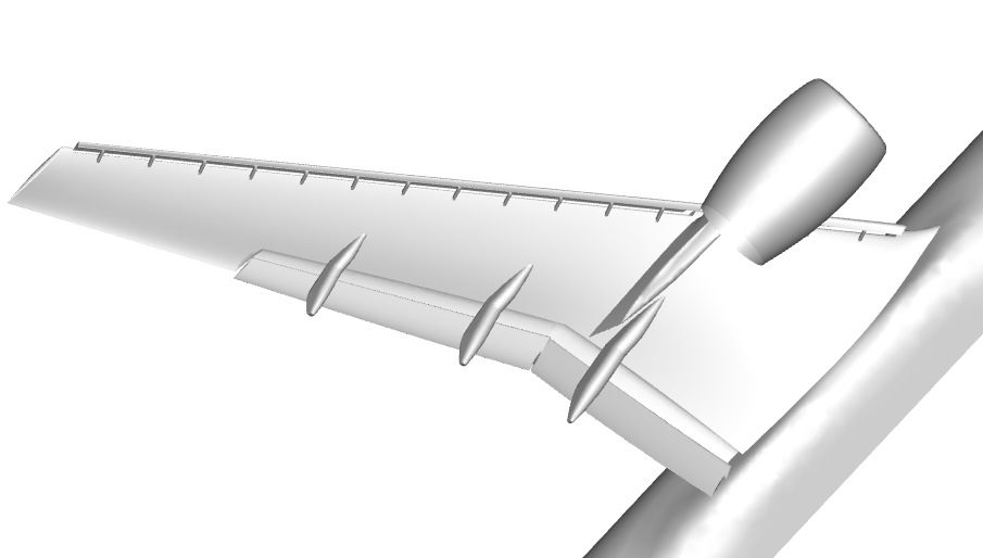 |
| The geometry of the high lift Common Research Model |
University of Kansas (KU) participated in two TFGs: High Order Discretization and WMLES. We learned a lot during the productive discussions in both TFGs. Our workshop results demonstrated the potential of high-order LES in reducing the number of degrees of freedom (DOFs) but also contained some inconsistency in the surface oil-flow prediction. After the workshop, we continued to refine the WMLES methodology. With the addition of an explicit subgrid-scale (SGS) model, the wall-adapting local eddy-viscosity (WALE) model, and the use of an isotropic tetrahedral mesh produced by the Barcelona Supercomputing Center, we obtained very good results in comparison to the experimental data.
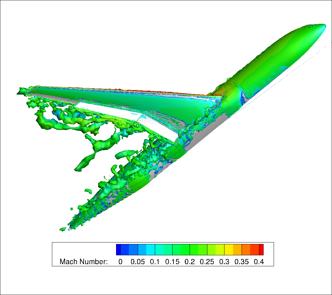
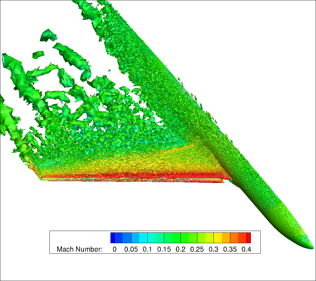
At the angle of attack of 19.57 degrees (free-air), the computed surface oil flows agree well with the experiment with a 4th-order method using a mesh of 2 million isotropic tetrahedral elements (for a total of 42 million DOFs/equation), as shown in the following figures. The pizza-slice-like separations and the critical points on the engine nacelle are captured well. Almost all computations produced a separation bubble on top of the nacelle, which was not observed in the experiment. This difference may be caused by a wire near the tip of the nacelle used to trip the flow in the experiment. The computed lift coefficient is within 2.5% of the experimental value. A movie is shown here.
 |
| Comparison of surface oil flows between computation and experiment |
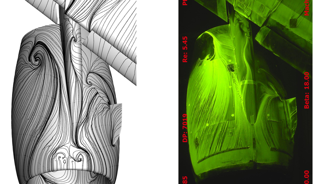 |
| Comparison of surface oil flows between computation and experiment |
Multiple international workshops on high-order CFD methods (e.g., 1, 2, 3, 4, 5) have demonstrated the advantage of high-order methods for scale-resolving simulation such as large eddy simulation (LES) and direct numerical simulation (DNS). The most popular benchmark from the workshops has been the Taylor-Green (TG) vortex case. I believe the following reasons contributed to its popularity:
Using this case, we are able to assess the relative efficiency of high-order schemes over a 2nd order one with the 3-stage SSP Runge-Kutta algorithm for time integration. The 3rd order FR/CPR scheme turns out to be 55 times faster than the 2nd order scheme to achieve a similar resolution. The results will be presented in the upcoming 2021 AIAA Aviation Forum.
Unfortunately the TG vortex case cannot assess turbulence-wall interactions. To overcome this deficiency, we recommend the well-known Taylor-Couette (TC) flow, as shown in Figure 1.

Figure 1. Schematic of the Taylor-Couette flow (r_i/r_o = 1/2)
The problem has a simple geometry and boundary conditions. The Reynolds number (Re) is based on the gap width and the inner wall velocity. When Re is low (~10), the problem has a steady laminar solution, which can be used to verify the order of accuracy for high-order mesh implementations. We choose Re = 4000, at which the flow is turbulent. In addition, we mimic the TG vortex by designing a smooth initial condition, and also employing enstrophy as the resolution indicator. Enstrophy is the integrated vorticity magnitude squared, which has been an excellent resolution indicator for the TG vortex. Through a p-refinement study, we are able to establish the DNS resolution. The DNS data can be used to evaluate the performance of LES methods and tools.

Figure 2. Enstrophy histories in a p-refinement study
Happy 2021!
The year of 2020 will be remembered in history more than the year of 1918, when the last great pandemic hit the globe. As we speak, daily new cases in the US are on the order of 200,000, while the daily death toll oscillates around 3,000. According to many infectious disease experts, the darkest days may still be to come. In the next three months, we all need to do our very best by wearing a mask, practicing social distancing and washing our hands. We are also seeing a glimmer of hope with several recently approved COVID vaccines.
2020 will be remembered more for what Trump tried and is still trying to do, to overturn the results of a fair election. His accusations of wide-spread election fraud were proven wrong in Georgia and Wisconsin through multiple hand recounts. If there was any truth to the accusations, the paper recounts would have uncovered the fraud because computer hackers or software cannot change paper votes.
Trump's dictatorial habits were there for the world to see in the last four years. Given another 4-year term, he might just turn a democracy into a Trump dictatorship. That's precisely why so many voted in the middle of a pandemic. Biden won the popular vote by over 7 million, and won the electoral college in a landslide. Many churchgoers support Trump because they dislike Democrats' stances on abortion, LGBT rights, et al. However, if a Trump dictatorship becomes reality, religious freedom may not exist any more in the US.
Is the darkest day going to be January 6th, 2021, when Trump will make a last-ditch effort to overturn the election results in the Electoral College certification process? Everybody knows it is futile, but it will give Trump another opportunity to extort money from his supporters.
But, the dawn will always come. Biden will be the president on January 20, 2021, and the pandemic will be over, perhaps as soon as 2021.
The future of CFD is, however, as bright as ever. On the front of large eddy simulation (LES), high-order methods and GPU computing are making LES more efficient and affordable. See a recent story from GE.

 |
| Figure 1. Various discretization stencils for the red point |


|
| p = 1 |
 
|
| p = 2 |
|
| p = 3 |
|
|
CL
|
CD
|
|
p = 1
|
2.020
|
0.293
|
|
p = 2
|
2.411
|
0.282
|
|
p = 3
|
2.413
|
0.283
|
|
Experiment
|
2.479
|
0.252
|

Author:
Allie Yuxin Lin
Marketing Writer
In today’s fast-paced and ever-evolving world, staying ahead requires more than just keeping up with the latest trends and technologies. It necessitates continuous learning and skill development, making training an essential component of personal and organizational growth. Whether you’re an individual looking to sharpen your skills or a business aiming to boost productivity, effective training can unlock a wealth of potential. At Convergent Science, we believe constant learning is an indispensable aspect of success that wields the power to transform your career or your company’s future. Our training sessions are where learning feels like an adventure, where every new skill is a boon, and where each attended course is a ticket to revealing your true abilities. In this blog, we will discuss the what, who, when, where, and why of our training program.
At Convergent Science, our training program is designed to get people familiar with our innovative, multi-purpose CFD solver, CONVERGE. Our courses are a way to get acquainted with our software and modeling options while working through a wide variety of example cases. In addition to our introductory training course, which serves as a gateway to CONVERGE, we also offer 10+ different application-focused trainings and 20+ different feature-focused training courses. Many of our sessions also include hands-on practice with our user-friendly GUI, CONVERGE Studio. If you’re looking for a little personalized help, we include a training course specifically so you can work one-on-one with a Convergent Science engineer on a case of your choosing. Additionally, if you don’t see the topic you’re looking for, or if you’d like to organize a training session just for your team, let us know! Our customized training lets you design your own session to best suit your specific needs. In other words, it’s an opportunity for you to tell us your vision of how we can best help you, and we’ll turn it into reality.

“The CONVERGE training I attended significantly enhanced my capability in performing high-fidelity FSI analyses, enabling me to accurately simulate complex phenomena and optimize compressor performance,” remarked Barkın Kılıç, Lead R&D Engineer at Beko. “The training provided invaluable insights into the advanced functionalities of CONVERGE, and the hands-on approach has greatly accelerated my company’s application of these tools in real-world R&D projects. The sessions have also paved the way for us to explore new avenues of research, allowing us to strive toward performance, efficiency, and sustainability targets with a higher degree of confidence.”
Everyone stands to benefit from one of our CONVERGE training sessions. Whether you’re a prospective client, existing academic or commercial user, new employee, or just an interested engineer, our courses are open to you. Here at Convergent Science, we believe learning is an inclusive experience.
“As a new user, I found CONVERGE’s interface to be fairly intuitive, but I wanted to master some of the additional features to advance my academic research. CONVERGE’s specialized training programs helped me accelerate my progress and provided a unique environment to learn directly from CONVERGE engineers and developers,” said Mickael M. Silva, Aramco Americas. “Now, with over half a decade of daily CONVERGE use, I still try to attend these training sessions whenever possible. They continue to be invaluable for exploring new features and deepening my understanding of complex model implementations and best practices. I definitely recommend the training sessions, for new and experienced users alike.”
We regularly offer free CONVERGE training sessions, taught by our expert engineers and covering a wide range of our software’s models and features, as well as how to apply them to specific applications. For the most part, we schedule the courses we are planning to offer in a given year at the end of the preceding year. The decision of which sessions to offer depends on the conferences we’ve attended over the past year, what our existing or prospective clients are interested in, and what topics are currently popular in the engineering community. Despite the schedule being determined well in advance, training sessions may be added or removed throughout the year, and scheduled sessions may be modified regarding the date, time, or content. Check out our website for the full schedule, and check back frequently to ensure you don’t miss any updates!
CONVERGE training is available in both live and on-demand formats. You can attend a live training online or in-person at one of our offices in the United States (Madison, Detroit, and Houston), Europe (Linz), and India (Pune). If you can’t make it to a live session, or you want to catch up on a topic, watch our on-demand training sessions, which are available 24/7 on the Convergent Science Hub. These pre-recorded courses provide you with an opportunity to learn CONVERGE anytime, anywhere. Log in or create an account today!
We built our training program to help the engineering community move forward by teaching them how to use a multi-purpose, state-of-the-art CFD software. With our expert engineers guiding them every step of the way, prospective and existing customers can get acquainted with our software to help them excel in their careers, and students and other academics can learn about features that will help them perform cutting-edge research.
“Participating in the CONVERGE training program has been an invaluable experience and a crucial step in gaining the expertise needed to learn CONVERGE’s capabilities and achieve reliable simulation results,” commented Andrea Piano, Assistant Professor at Politecnico di Torino. “The training provided technical knowledge, the chance to interact and exchange ideas and best practices with CONVERGE experts, and, last but not least, a possibility for networking with colleagues from industry and academia.”

Author:
Elizabeth Favreau
Marketing Writing Team Lead
In today’s energy and transportation industries, sprays and combustion are at the heart of many of our most relied-upon technologies. From internal combustion engines to gas turbines to burners, better understanding the fundamental physical processes that drive these devices can help us make them more efficient and more sustainable in the future.
Professor Noah Van Dam’s Multi-Phase and Reacting Flows Laboratory at the University of Massachusetts Lowell is dedicated to studying and characterizing these processes through computational fluid dynamics (CFD) modeling. A CFD aficionado since his undergraduate days, Prof. Van Dam was introduced to CONVERGE during his postdoctoral studies at Argonne National Laboratory, where he focused on the effects of fuel properties on engine performance. When he started his own lab at UMass Lowell, he continued to use CONVERGE through the CONVERGE Academic Program, which provides licenses, training, and support for academic research.
CONVERGE wasn’t the only thing Prof. Van Dam carried over into his lab at UMass Lowell—he also continued his research on spray and combustion modeling. When Aman Kumar joined Prof. Van Dam’s lab in 2020 as a graduate research assistant, he began conducting detailed numerical studies of the Engine Combustion Network (ECN) Spray G injector. He was interested in understanding how the injector geometry and the location of the spray plume affected downstream conditions and overall engine performance.
“I’ve been focusing on fundamental studies, because everything starts right at the beginning with how you are injecting the fuel and how the mixture is being developed,” Aman said. “If the mixture is homogenous, the fuel-air mixture will burn at reduced combustion temperature and the engine will produce lower amounts of NOx, soot, and particulate matter emissions.”
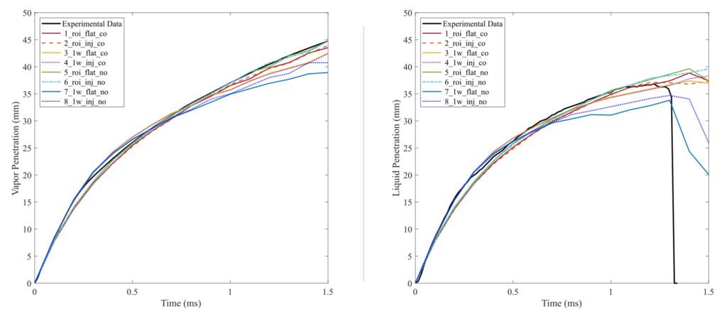
In his studies, Aman experimented with both Reynolds-Averaged Navier-Stokes (RANS)1 and large eddy simulation (LES)2 modeling frameworks. He looked at various parameters, including having the injector tip geometry drawn in the cylinder head versus not including it, initializing the parcels at the counterbore exit versus the nozzle exit, using an experimentally derived rate of injection versus reading the injector flow parameters from a volume of fluid (VOF) simulation of the internal injector flow, and the use of a nominal versus x-ray scanned injector geometry. He compared spray penetration and other global parameters to experimental data. Figure 1 shows vapor and liquid penetration length plots for eight RANS simulation cases compared to experimental data. The different cases resulted in only slightly different penetration lengths, and the CONVERGE simulations matched well with the experimental data. Figure 2 shows a comparison of projected liquid volume fraction for the RANS and LES cases. While the RANS simulation captures the global spray behavior, the LES simulation better captures the local turbulent flow features.
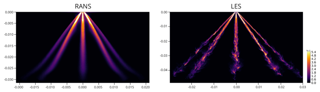
Following their Spray G studies, Aman and Prof. Van Dam turned their attention to alternative fuels, in particular ammonia.
“Our future energy requirements need to move in a direction where we’re reducing the net greenhouse gases that we are emitting from transportation and other energy systems. Alternative fuels, such as ammonia, is one pathway that has been proposed, and it’s one that is looking more and more like it is going to be a fruitful avenue for research and actual production,” explained Prof. Van Dam.
The properties of ammonia, however, differ significantly from traditional hydrocarbon fuels. For example, liquid ammonia sprays are more likely to undergo flash boiling under most engine operating conditions, which could necessitate new injection strategies. Aman used CONVERGE to study how well current spray models can capture liquid ammonia spray behavior.3
He used a RANS turbulence model with two different simulation methods: a VOF approach for in-nozzle simulations and a Lagrangian-Eulerian (LE) parcel-based approach for downstream simulations. For the LE simulations, Aman also tested two different methods of initializing the spray parcels: one-way coupling using the results from the in-nozzle simulations and a prescribed rate-of-injection (ROI) method.
Figure 3 compares experimental images with simulated ammonia sprays using the in-nozzle VOF approach at different pressure ratios. The CONVERGE simulations are able to capture the widening of the spray plume as the spray begins to undergo flash boiling at higher pressure ratios.
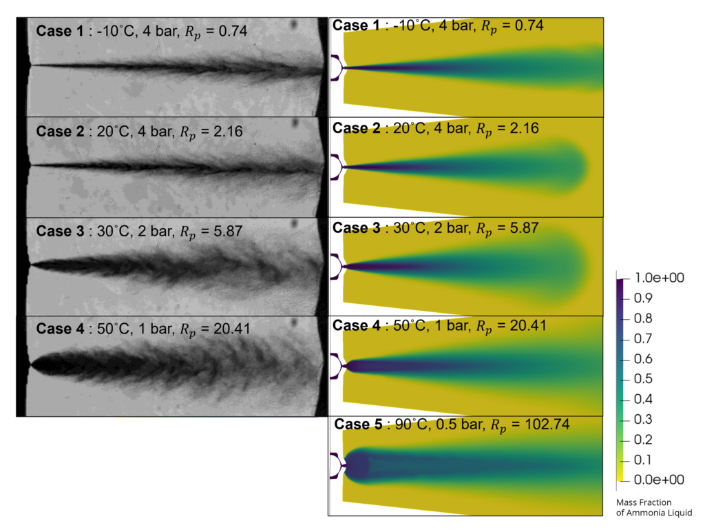
Aman found that for a non-flashing case, the two LE modeling frameworks best captured the liquid penetration lengths, whereas the VOF in-nozzle method performed the best for the flash-boiling case. A significant amount of ammonia vapor is produced inside the counterbore geometry which can be seen easily in CFD simulations but is difficult to capture in experiments. He and his lab are continuing their studies into ammonia sprays and are working to further improve the existing spray models to robustly capture ammonia’s flash boiling behavior.
As mentioned earlier, fuel injection is only the beginning of the story in an IC engine. Continuing on downstream, Prof. Van Dam is also investigating the combustion of alternative fuels. For these studies, Prof. Van Dam teamed up with other researchers including Prof. Dimitris Assanis at Stony Brook University with the goal of gaining a better understanding of ammonia/hydrogen combustion.
As combustible fuels go, both ammonia and hydrogen come with some challenges. Ammonia is hard to ignite and has a very low flamespeed. On the other hand, hydrogen is very reactive and burns very rapidly.
“By mixing hydrogen and ammonia, we can mitigate some of the issues of each individual fuel and create a blended fuel that behaves much more closely to our current hydrocarbon fuels. We have a lot of experience with hydrocarbon fuels, and so it’s much easier for us to design engines for fuels that behave similarly,” said Prof. Van Dam.
In their collaborative study,4 the researchers from UMass Lowell and Stony Brook first tested several different chemical kinetic mechanisms for ammonia/air and ammonia/hydrogen/air combustion to determine which mechanism best matched available experimental data for laminar flamespeed and ignition delay. They then took the best performing mechanism and ran 3D CFD simulations in CONVERGE to study the combustion characteristics. Figure 4 shows a visual comparison of the flame from experimental Schlieren images and the CFD results for ammonia/air combustion. The simulations show similar flame shapes as the experiment at each time step for all three equivalence ratios.
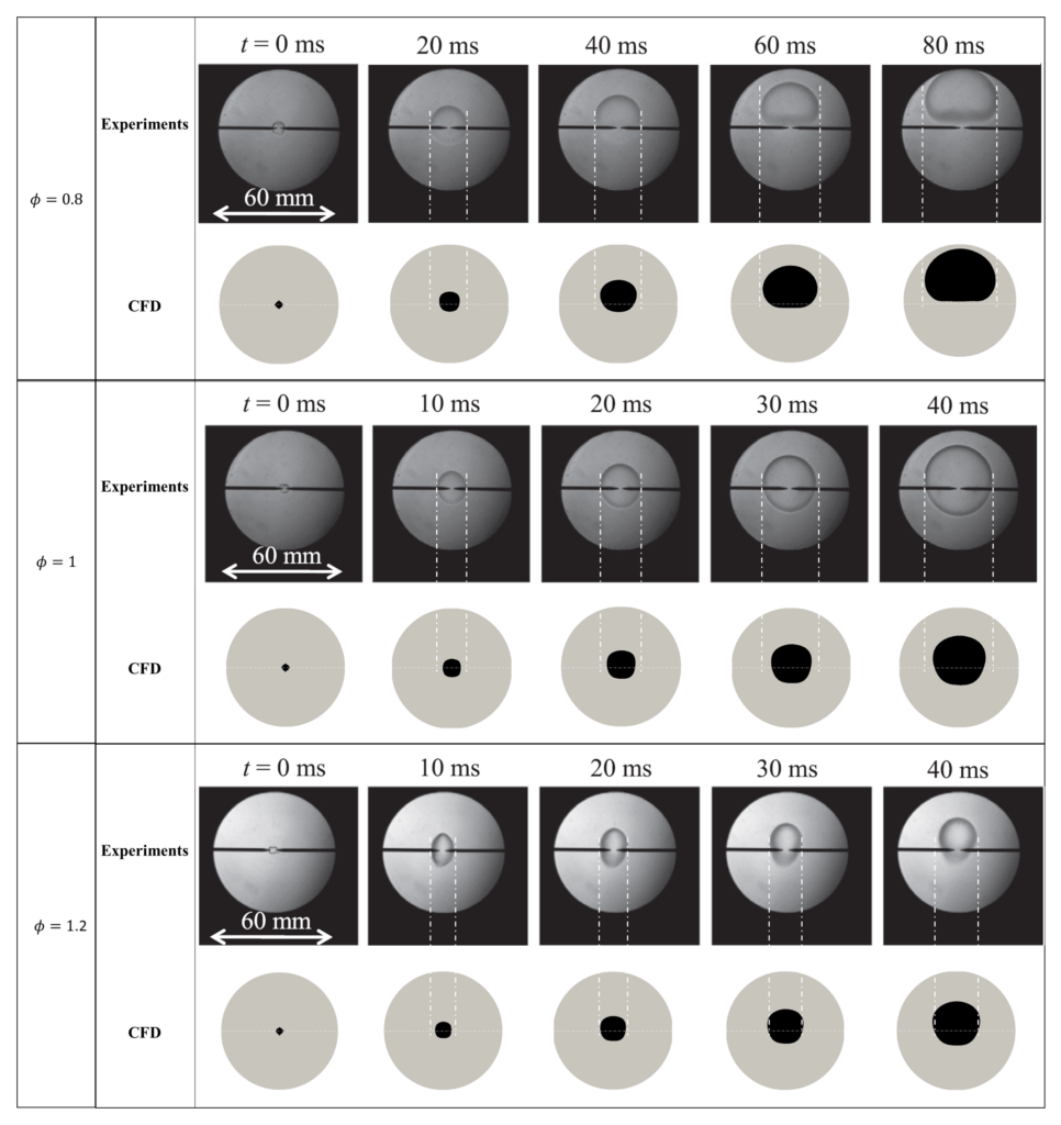
The researchers discovered that compared to ammonia/air combustion, the ammonia/hydrogen/air combustion resulted in a faster flame that was less dependent on the spark event and did not experience buoyancy effects. They concluded that ammonia/hydrogen mixtures demonstrate complementary combustion characteristics that could lead to improved performance for engine applications.4
The group from UMass Lowell and Stony Brook are continuing their research into ammonia combustion, which you can look forward to in an upcoming paper at the 2024 ICE Forward Conference.5
Alternative fuels aren’t the only pioneering technology that Prof. Van Dam’s lab is researching—they are also helping to develop reliable propulsion systems for the next generation of unmanned surface vessels. In a collaborative project with the U.S. Office of Naval Research, Prof. Van Dam’s group is investigating how burners operating in marine environments are affected by intaking salty air.
Undergraduate researcher Colin Wildman began working on this project when he joined Prof. Van Dam’s lab in 2022. The first step for the project was to test different diesel fuel surrogates in a swirl burner to determine which one most accurately represented the flame shapes and emissions of the experimental setup. Using the SAGE detailed chemistry solver and LES turbulence modeling, Colin tested five different diesel fuel surrogates (Surrogate A, Surrogate B, T15, T15 + CH5, and T20).6 He also tested a more computationally efficient RANS turbulence model, using Surrogate A, to see if that would give them reasonable results in a shorter amount of time. Figure 5 shows the temperature contours of the resulting flames for the different surrogates they tested. The RANS model produced a smoother, more cylindrical flame shape compared to the LES simulations, which more accurately captured the intricate flame structures. Because of this, they decided to stick with LES modeling with diesel Surrogate A. The next step in this project is to introduce salt into the flame and see how that affects combustion and emissions production.
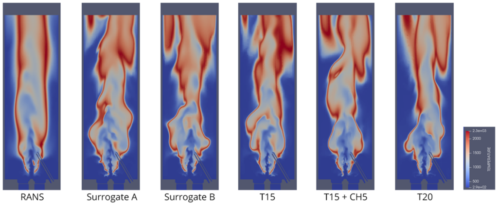
When Colin joined Prof. Van Dam’s lab, he had no experience with CFD software. By watching our on-demand training courses, getting hands-on experience with CONVERGE, and working with our support engineers, he was able to become a proficient and independent CFD user.
“The CONVERGE Academic Program, with the training videos and support, has helped me grow into a student that’s independent. It’s kind of a happy memory for me thinking that when I started, I had no idea what I was doing. And now I’m independent, running cases on my own. Now when we have new students join the lab, I’m the one that shows them the ropes,” Colin said.
The goal of the CONVERGE Academic Program is to equip students and other academic researchers with the tools and skills they need to succeed in academia and beyond. Academic users get access to the full-featured CONVERGE package, which helps prepare them for a smooth transition to a career in industry after graduation. Stories like Colin’s emphasize that with the right resources and support, learning an advanced CFD software and conducting impactful, cutting-edge research is well within your reach.
To learn more about the CONVERGE Academic Program, visit our webpage or fill out this form to get in touch with our academic specialists!
[1] Kumar, A. and Van Dam, N., “Study of Injector Geometry and Parcel Injection Location on Spray Simulation of the Engine Combustion Network Spray G Injector,” Journal of Engineering for Gas Turbines and Power, 145(7), 2023. DOI: 10.1115/1.4062414
[2] Kumar, A., Boussom, J.A., and Van Dam, N., “Large-Eddy Simulation Study of Injector Geometry and Parcel Injection Location on Spray Simulation of the Engine Combustion Network Spray G Injector,” Journal of Engineering for Gas Turbines and Power, 146(8), 2024. DOI: 10.1115/1.4063957
[3] Kumar, A. and Van Dam, N., “Liquid Ammonia Sprays for Engine Applications,” ILASS-Americas 34th Annual Conference on Liquid Atomization and Spray Systems, Ithaca, NY, United States, May 19–22, 2024.
[4] Shaalan, A., Nasim, M.N., Mack, J.H., Van Dam, N., and Assanis, D., “Understanding Ammonia/Hydrogen Fuel Combustion Modeling in a Quiescent Environment,” ASME 2022 ICE Forward Conference, ICEF2022-91185, Indianapolis, IN, United States, Oct 16–19, 2023. DOI: 10.1115/ICEF2022-91185
[5] Mathai, J.R., Rana, S., Shaalan, A., Nasim, M.N., Trelles, J.P., Mack, J.H., Assanis, D., and Van Dam, N., “Numerical Study of Buoyancy and Flame Characteristics of Ammonia-Air Flames,” 2024 ASME ICE Forward Conference, ICEF2024-141569, San Antonio, TX, United States, Oct 20–23, 2024. (Forthcoming)
[6] Wildman, C., Fernandez, J., and Van Dam, N., “Low-Pressure Swirl Burner for Marine Propulsion Applications,” 2023 CONVERGE CFD Conference, Online, Sep 26–28, 2023.
Author:
Elizabeth Favreau
Marketing Writing Team Lead
The need to reduce emissions from the transportation sector has spawned a new era of evolution and development in the automotive industry. Many countries around the world have identified electric vehicles as a crucial piece of the decarbonization puzzle, and as with any emerging technology (or, more precisely in the case of electric vehicles, reemerging), safety is a primary concern.
While statistically the safety of electric vehicles is on par with conventional powertrains, battery thermal runaway and thermal propagation have been thrust into the spotlight as a potential hazard. In the worst-case scenarios, thermal propagation can lead to battery fires or explosions, which pose a threat to vehicle occupants and can release toxic gases into the environment.
Convergent Science recently teamed up with IAV to take on the problem of thermal runaway propagation. IAV is an international company based in Berlin, Germany, that has been developing technical solutions for the automotive industry for over forty years. They are dedicated to providing the best expertise and methodologies to their customers to help them tackle challenging engineering problems, such as thermal propagation in electric vehicle batteries.
“There are many reasons why it’s important to study thermal propagation,” says Dr. Alexander Fandakov, who leads the R&D team working on battery electric vehicle powertrain development at IAV. “First and foremost is the safety of the vehicle, but another big reason is legislation.”
Many jurisdictions around the world have enacted legislation stipulating that if damage to the electric vehicle battery is imminent, there must be sufficient time for drivers and passengers to stop and exit the vehicle before thermal propagation occurs. For example, UN regulations require that vehicle occupants receive a signal “5 minutes prior to the presence of a hazardous situation inside the passenger compartment caused by thermal propagation”.1 Moreover, there has been discussion in some jurisdictions about significantly increasing the duration of time required between thermal runaway and thermal propagation, which would essentially mean that no thermal propagation would be allowed.
To meet these legislative requirements, manufacturers must conduct extensive testing of their battery modules or packs under different conditions to evaluate the risk of thermal runaway and devise methods to mitigate thermal propagation. Extensive testing, however, doesn’t come cheap.
“The problem with electric vehicle battery development is that when you want to perform testing related to thermal propagation, you generally need at least a module, or the entire battery pack, which typically are not available until a late stage of the development process. And when looking into thermal propagation, you have to consider different boundary conditions, and then you basically put the battery pack in the trash after the test. So these tests are very, very expensive,” Alexander explains, “and the implementation of additional propagation mitigation measures based on the test results are typically anything but straightforward at this late development stage.”
It follows naturally, then, that if you can cut down on the number of physical tests, you can save a significant amount of time and money. This is where computational fluid dynamics (CFD) comes into play. CFD allows engineers to simulate battery packs with different chemistries, materials, and configurations under different conditions to virtually assess the efficacy of thermal propagation mitigation strategies. To be an effective development tool, however, you need to have a predictive CFD code—which is why IAV elected to use CONVERGE.
“CONVERGE uses a physics-based approach to model 3D thermal runaway and thermal propagation,” says Kislaya Srivastava, Principal Engineer at Convergent Science. “This means that we don’t rely on experimental profiles, instead using chemical reaction mechanisms coupled with high-fidelity models to predict the thermal runaway behavior.”
IAV and Convergent Science worked together to develop and validate a numerical approach in CONVERGE to simulate thermal propagation, starting with modeling the thermal runaway kinetics of different battery chemistries, then using the validated kinetic mechanisms to predict the 3D spatial temperature distributions and heat transfer in battery systems employing a variety of different materials. In this blog post, we’ll take a look at an overview of the team’s 3D modeling work; for details on the experimental work and more in-depth information on the simulation studies, please refer to Sens et al. 2024.2
The team from IAV and Convergent Science first used CONVERGE to conduct single-cell tests of different lithium-ion battery chemistries, including nickel manganese cobalt (NMC) and lithium iron phosphate (LFP), as well as a sodium-ion battery (SIB). Figure 1 shows the single-cell geometry, including clamps, used for the 3D CONVERGE simulations.
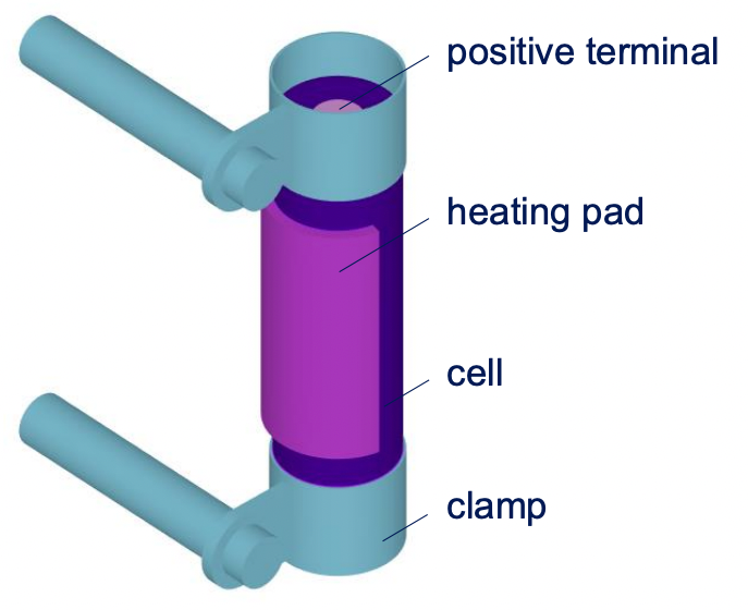
The cell is modeled as a single solid with an applied anisotropic thermal conductivity along the direction of the cell layers, and interfaces are defined between the components depicted in Figure 1 to allow heat transfer between them. The team used established thermal runaway mechanisms available in CONVERGE and calibrated them to accurately represent the thermal abuse within the cell.
In this blog post, we’ll focus on an NMC811 cell, for which the team employed the Ren mechanism.3 The team calibrated the mechanism using experimental data from a constant heating test, then validated the NMC model with the calibrated mechanism against experimental data from heat-wait-seek and nail penetration tests.
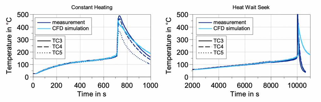
Figure 2 compares the CONVERGE results with measurement data from three thermocouple positions for the constant heating and heat-wait-seek tests. Figure 3 shows the results of the nail penetration test, comparing CONVERGE with measurement data from the most representative thermocouple position. The CONVERGE results match well with the experimental data in all three cases, demonstrating that the calibrated mechanism is able to represent the thermal runaway behavior of the cell for different initiation methods, thus confirming its predictivity.
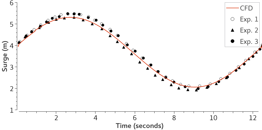
With the single-cell validation completed, the team moved on to conduct thermal propagation studies in a seven-cell module, as shown in Figure 4. They employed the same calibrated Ren mechanism for the NMC811 cell chemistry from their single-cell studies. They looked at several different scenarios, including where the space around the cells within the housing was filled with either nitrogen or air, and the application of an insulating inter-cell element or immersion oil cooling to delay thermal propagation.
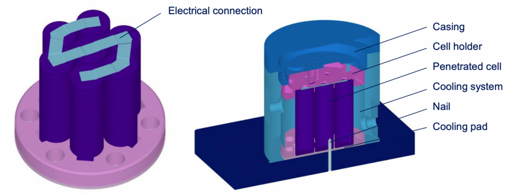
“In addition to the thermal runaway chemistry, CONVERGE offers a number of features that make these simulations possible,” says Kislaya. “CONVERGE’s autonomous meshing easily handles the complex battery pack geometries with no user meshing time, and Adaptive Mesh Refinement dynamically adjusts the mesh throughout the simulation to capture the complex physical phenomena at a lower computational cost. In addition, CONVERGE’s conjugate heat modeling allows us to analyze heat transfer between the solid and fluid domains, and its multi-phase modeling capabilities enable us to investigate liquid cooling techniques.”
Figure 5 shows the results for a case with air surrounding the cells and no thermal insulation applied. Thermal runaway is initiated in the center cell (cell 7) via nail penetration; the adjacent cells also go into thermal runaway immediately after the nail penetration occurs. CONVERGE is able to capture the timing and duration of the thermal propagation very well. While the predicted peak temperatures are lower than the measured peak values, the measured peak temperatures are considered mainly as gas temperatures and thus cannot be directly compared with the solid cell surface temperatures obtained from the simulation. The solid cell surface temperatures drive the processes inside the cell that ultimately result in thermal runaway, and the simulation captures these important values.
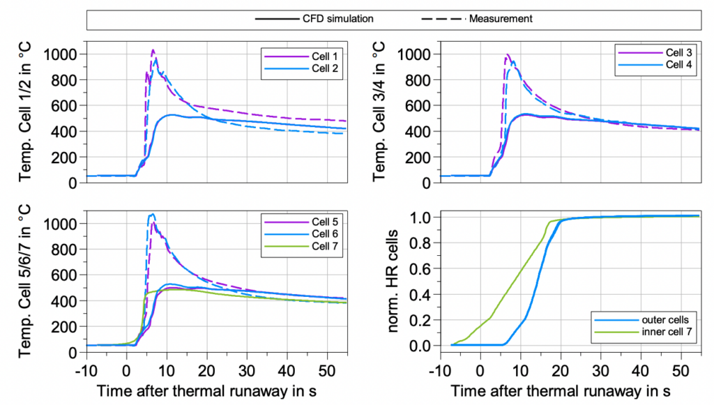
After validating the CONVERGE model for a case with immediate thermal propagation, IAV turned their attention to mitigation strategies. In this post, we’ll focus on the adoption of an insulating inter-cell element, but the results of oil cooling can also be found in Sens et al. 2024.2
“One way you can prevent heat from transferring from one cell to another is by inserting a foam, for example, that is a thermal insulator between the cells,” says Alexander. “But such a foam also has challenges because it has an impact on the overall weight of the battery, it has an impact on cost, and so on. It’s a very complex problem, and that’s why it is crucial to be able to investigate different types of inter-cell materials with simulation.”
Figure 6 shows the impact of adding an inter-cell element on thermal propagation. Thermal runaway is once again triggered in the center cell (cell 7) via nail penetration. As you can see, the addition of the inter-cell element significantly delays thermal propagation to the adjacent cells. Overall, the CONVERGE simulations are able to represent well the progression of the thermal propagation, especially considering the immense complexity of the events occurring in the experimental setup that are not considered in these simulations, such as mechanical deformation, material melting, and material ejection out of the battery. The deviation between the measured and simulated total propagation duration is approximately 10%.
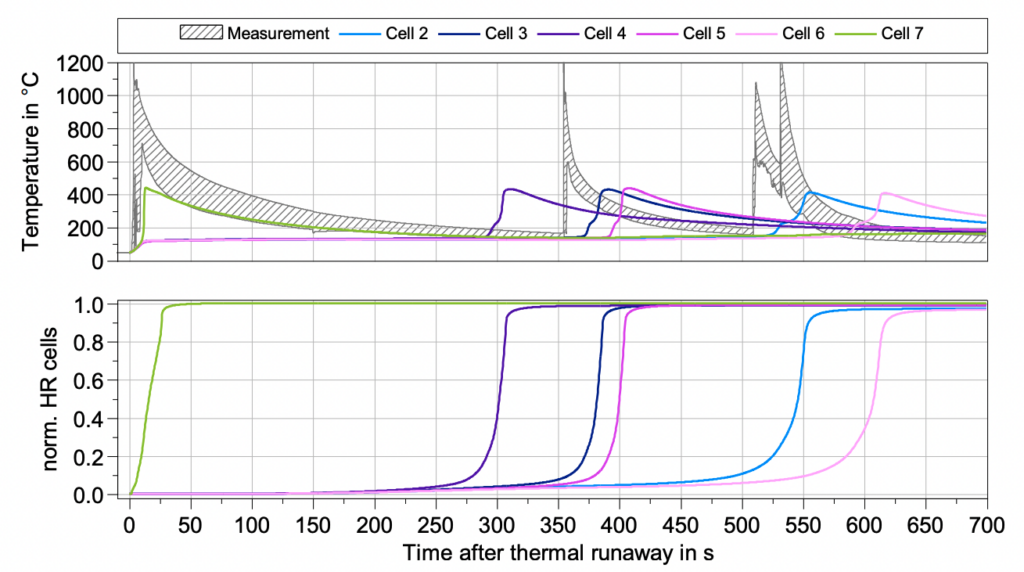
This successful collaboration brought together IAV’s extensive industry expertise and state-of-the-art testing facilities with CONVERGE’s predictive simulation capabilities. Together, IAV and Convergent Science developed and validated a numerical model to study thermal runaway and thermal propagation in battery modules. In the future, this methodology can be applied to different battery chemistries, module configurations, and thermal propagation mitigation strategies. Having a powerful and efficient method to study thermal propagation is a game-changer for industry, enabling manufacturers to meet legislative requirements and ensure the safety of electric vehicles for consumers, all while saving time and reducing development costs.
Learn more about this collaborative work in our joint webinar: A Cool Take on Hot EV Batteries: Navigating Thermal Propagation With CFD Based on Thermal Runaway Kinetics Modeling.
[1] United Nations, “UN Regulation No 100 – Uniform Provisions Concerning the Approval of Vehicles With Regard to Specific Requirements for the Electric Power Train,” E/ECE/Rev.2/Add.99/Rev.3.
[2] Sens, M., Fandakov, A., Mueller, K., von Roemer, L., Woebke, M., Tourlonias, P., Mueller, T., Burton, T., Srivastava, K., and Senecal, P.K., “From Thermal Runaway to No Thermal Propagation,” 45th International Vienna Motor Symposium, Vienna, Austria, Apr 24–26, 2024.
[3] Ren, D., Liu, X., Feng, X., Lu, L. Ouyang, M., Li, J., and He, X., “Model-Based Thermal Runaway Prediction of Lithium-Ion Batteries From Kinetics Analysis of Cell Components,”Applied Energy, 228, 633-644, 2018.
If you’ve ever talked to someone who works at Convergent Science, you will undoubtedly have heard us extolling the virtues of CONVERGE’s autonomous meshing. Got a complicated geometry? No problem! Moving boundaries? Easy! No time to waste on meshing? We’ve got you covered!
This enthusiasm, we would argue, is not unwarranted—CONVERGE’s autonomous meshing strategy was truly a novel innovation. So much so that when CONVERGE was first released, the Convergent Science founders were met with more than a little skepticism. As Convergent Science Co-Founder Kelly Senecal puts it, “Nobody believed us.” The founders had to prove the worth of this new feature, asking companies to provide their hardest geometry so they could see for themselves that, in a matter of minutes, the geometry could be up and running in CONVERGE.
Fast forward 16 years, and CONVERGE’s autonomous meshing has become the industry gold standard. As other CFD solvers are releasing their own versions of automated meshing, I wanted to find out what it is that makes CONVERGE’s autonomous meshing different. To do so, I sat down and talked with Kelly, one of the original developers of CONVERGE and, arguably, the number one fan of autonomous meshing.
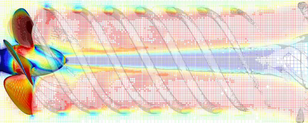
To start off, what exactly is autonomous meshing?

Autonomous meshing is truly automated meshing, in the sense that the user just has to supply a few parameters in the user interface, and all the actual meshing is done at runtime by CONVERGE. So it takes the meshing completely out of the hands of the user. You still have control over the mesh, though. As a user, you can define fixed embedding regions if you know ahead of time that you want to have fine resolution near a boundary, for example. CONVERGE also uses Adaptive Mesh Refinement—at every time-step the code is intelligently figuring out where mesh is needed and where mesh can be removed based on the flow physics to be very efficient with the cell count.
What prompted you, Keith, and Eric to develop an automated meshing approach?
We spent a lot of time during our graduate school days, and during the early days of Convergent Science back when it was a consulting company, making meshes for people in a code called KIVA. And even though we could do it relatively quickly—we had created tools to help us—it could still take days or even weeks to make a mesh for a complicated geometry. And when you’re an engineer, you want to spend your time running your CFD simulations, analyzing results, and using them to make design decisions; you don’t want to spend all your time making meshes. So that’s what motivated us. We thought there had to be a better way.
What was the process like writing the code for autonomous meshing?
That’s a good question. Scary? Because we didn’t know if it was going to work or not. And we had some missteps. We originally based the code around an immersed boundary method, as opposed to the modified cut-cell Cartesian approach we use now. We thought the immersed boundary method could work, and we got something running—not quickly exactly, it probably took a year and a half to get the code up and running for a 3D engine simulation. But we realized it wasn’t going to work because it was hard to get that approach to conserve robustly. So we had to scrap essentially all the code we had written and go to this new approach. So that was a bit scary. And we still weren’t sure the new method was going to work. Originally, the automated meshing took minutes or even hours to create the mesh in the solver. We get that question a lot: “Doesn’t this take forever?” And originally, yes it did. One of the real breakthroughs we came up with was making that process almost instant. It adds very little time to the overall CFD calculation, even though we’re remaking the mesh entirely at each time-step. Once we had that eureka moment, we knew we were onto something big. And so it went from scary to very exciting.
What makes CONVERGE’s autonomous meshing capabilities unique?
A lot of CFD codes these days throw around the automated meshing terminology fairly loosely, I would say. There are different levels of automated meshing out there, and how truly automated it is depends on a lot of factors, like how complicated your geometry is and whether or not you have moving boundaries. There are some codes that can do automated meshing for certain cases, but it’s really hard to be able to have automated meshing work in general for all cases. But that’s what we have. We have yet to find a case where we throw a geometry at CONVERGE and it isn’t able to mesh it. And so that’s what makes us unique—we have truly autonomous meshing for every case, no matter how complicated the geometry or the motion profiles are.
What kinds of practical benefits do companies see as a result of CONVERGE’s autonomous meshing?
Really it’s about efficiency. Maybe you have a design out in the field that is having problems, and you want to use CFD to figure out what happened. Or maybe you want to design a brand new flow device from scratch using CFD. In the past, you’d spend a lot of time just making your mesh. And once you’ve made your mesh, the next question is, “How do you know if it’s fine enough? How do you know that you’re grid-converged?” It’s very hard to answer that question with traditional meshing techniques, because it’s so difficult to make the mesh in the first place, you’re probably not going to want to make another one. With autonomous meshing in CONVERGE, it’s very easy to make multiple meshes and show grid convergence. So again, it makes the process much more efficient. It also gives you confidence in your solutions because you can very easily double or triple the resolution and see how that affects your answer. Of course, you still have to run those simulations, so that takes some computer time. But the actual engineer time is minimal. So it’s much more efficient, you’re more confident in your solutions, and you get more accurate results. And in the end, that leads to a better design.
What applications benefit the most from autonomous meshing?
The ones that benefit the most are cases with complicated geometries and moving boundaries. That’s what’s hardest to do traditionally in CFD, and most real fluid devices are complicated. There are approaches that can handle moving geometries, but a lot of them add numerical error because you’re deforming the mesh near the boundary, for example. Whereas with our autonomous meshing technique, we recreate the mesh at every time-step while the motion is occurring, so we avoid those numerical artifacts. Autonomous meshing can also handle large differences in scales—maybe you have really tiny channels in your geometry as well as very large areas. CONVERGE can handle those very different scales efficiently, automatically putting fine resolution in the small channels and very coarse resolution in the large areas. So varying scales, complicated geometries, and moving boundaries benefit the most. But again, even simple geometries benefit because you’re not spending any time making the mesh.
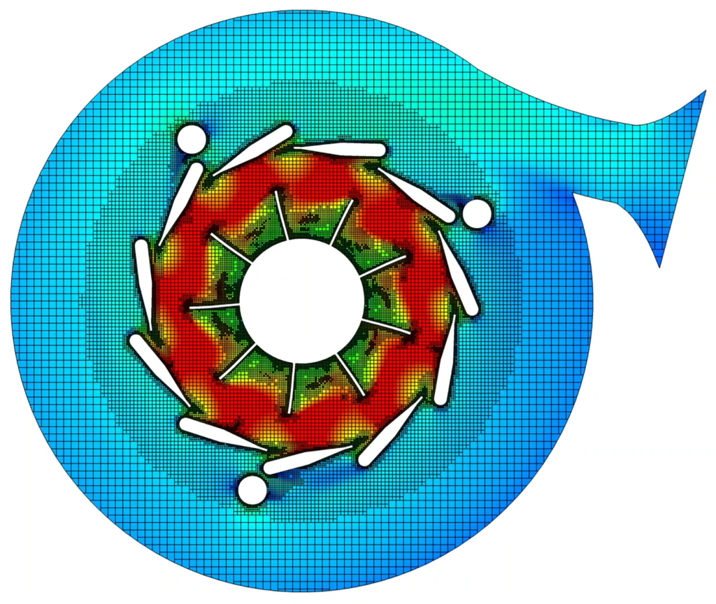
Are there any new meshing features currently in the works for CONVERGE?
In version 3.0, we released something called inlaid meshing. It’s not required for any simulation, but if you want to add a boundary layer mesh or a non-Cartesian mesh in a portion of your domain, you can do that through inlaid meshing. We already have all the tools implemented in the code to read those meshes and have them interface with the traditional cut-cell Cartesian mesh. What we’re working on now is automating the inlaid mesh generation similar to how we automate our traditional CONVERGE meshing. When this feature is implemented, the inlaid meshing will also be fully autonomous.
If someone is interested in trying autonomous meshing out for themselves, what should they do?
Reach out to us! We have a variety of licensing options available, whether you want to use CONVERGE for commercial purposes, to conduct academic research, or to learn a new skill for your resume. We also offer on-demand licensing and access to computing hardware through our cloud computing platform, CONVERGE Horizon. We would love to work with you to find the right license for your needs so you can experience the power of autonomous meshing for yourself!


The heartbeat of the global economy is commercial vehicles, and as the economy grows, so does the demand for on-road trucks, off-road construction equipment, and agricultural vehicles. These vehicles are almost entirely powered by compression ignition engines using fossil diesel fuel. In the face of the global climate crisis, this presents a real challenge: how do we provide efficient and productive commercial vehicle powertrains while reducing criteria and greenhouse gas (GHG) emissions? Full electrification of these vehicles faces many hurdles, such as cost, weight, operating hours, lack of infrastructure, and time to implementation. Thus, the most pragmatic and impactful way to reduce emissions in the near term is by using lower carbon intensity fuels, such as ethanol, methanol, natural gas, propane, hydrogen, or ammonia.

Using these fuels in heavy-duty engines as a substitute for diesel fuel is very challenging, because these fuels are poor direct replacements for diesel fuel. These fuels all have very low cetane numbers, which means they are very hard to autoignite and more suitable to spark ignition (SI) engines. But SI engines are NOT suited to heavy-duty applications because of the knock-limited peak torque, potential for catastrophic pre-ignition when highly boosted, poor torque density, poor torque response, low thermal efficiency, high exhaust temperatures, and high heat rejection. The combustion process used in conventional diesel engines is lean, mixing-controlled combustion (MCC). It is highly desirable for heavy-duty vehicles to use an engine that employs this combustion strategy—regardless of the fuel—because the engine will maintain the performance and operational characteristics of a diesel engine, such as high efficiency, no fear of knock or pre-ignition, snap torque, high torque at low speed, low cyclic variability, and robust combustion. An engine that has these characteristics, we like to say, “runs like a diesel”, which all stems from the mixing-controlled combustion process. Thus, an innovative combustion system is needed that will allow low-cetane fuels to ignite readily and be used in a non-premixed MCC strategy, just like the diesel engine today.
Using the CONVERGE computational fluid dynamics (CFD) modeling software, our engine combustion research group at Marquette University has been working to develop such an innovation known as prechamber enabled mixing-controlled combustion (PC-MCC). Illustrated in Figure 1, the concept uses a conventional compression ignition engine with high-pressure direct injection and adds an actively fueled prechamber igniter. The igniter contains a fuel injector, a spark plug, a small prechamber volume, and orifice passageways between the prechamber and main chamber. The high-pressure direct injector and prechamber injector use the same low-cetane fuel source. Figure 2 shows the operational strategy of PC-MCC with ethanol fuel compared to conventional diesel combustion (CDC). During the compression stroke, the prechamber is fueled with ethanol, while air from the main chamber is forced into the prechamber by piston motion. Closely coupled to the direct injection timing near top dead center, the prechamber is sparked, and the prepared charge is burned by rapid flame propagation. This combustion process elevates the pressure of the prechamber and promotes hot jet flames that are ejected into the main chamber. The penetrating jets impinge and subsequently ignite the direct-injected ethanol fuel, which would otherwise not autoignite.

As shown in Figure 3, the direct-injected ethanol, once ignited by the prechamber jet flames, burns in a mixing-controlled manner with a rate of combustion like that of diesel fuel. This is the ultimate goal: to allow the engine to “run like a diesel” by reproducing the diesel engine combustion process, but running on low-cetane fuels like ethanol, methanol, or even hydrogen and ammonia.

An animation of the CFD-predicted PC-MCC combustion process with ethanol fuel is illustrated in Figure 4. The prechamber jet flames are ejected toward the direct-injected ethanol fuel, igniting the ethanol fuel sprays very quickly and establishing a mixing-controlled, diffusion-style combustion process that is typical of a modern diesel engine.
This concept is currently under development with the assistance of two federal grants. The first is from a United States Department of Energy Vehicle Technologies Office award (DE-EE0009872), where the concept is being developed to convert diesel engines to be flex-fuel and run on gasoline/ethanol, while maintaining performance and dramatically reducing GHG emissions. The second is from the Advanced Research Projects Agency Energy’s (ARPA-e) REMEDY program (DE-AR0001528), which aims to reduce methane emissions, a powerful GHG, from natural gas engines by radically changing the combustion process to PC-MCC. The institutions working on these projects together with Marquette University are John Deere, Mahle Powertrain, the University of Wisconsin-Madison, Czero, ClearFlame Engines, and the Missouri Corn Merchandising Council. The CFD modeling has led to several publications by the team, showing how the CONVERGE simulations were used to determine the prechamber’s characteristics—such as volume, number of holes, hole size, and jet targeting—and the general PC-MCC operating strategy for prechamber fueling, injection timing, spark timing, and direct injection timing [1-5].
The modeling tools provided by CONVERGE were quintessential for performing the detailed CFD modeling needed to develop this advanced combustion concept. CONVERGE’s automatic mesh generation dramatically reduces the simulation setup time and complexity, allowing for rapid simulation development and analysis with confidence in the meshing strategy. Further refinement to the mesh is achieved through fixed grid embedding in user-defined regions of interest within the domain and CONVERGE’s Adaptive Mesh Refinement (AMR), which is able to resolve cell-to-cell gradients in temperature and velocity. AMR is especially useful when modeling the combustion process within the prechamber, the resultant high-intensity jets, and subsequent jet-spray induced combustion process. The predicted combustion process is captured using CONVERGE’s detailed chemical kinetics solver SAGE, which is fully coupled to the flow solution for accurate results and efficient solution times.
Based on the CFD modeling, a prototype PC-MCC engine was constructed and tested separately on pure ethanol fuel and natural gas, demonstrating a robust mixing-controlled combustion process with both fuels and highlighting the fuel-agnostic nature of the technology. Photos of the prototype hardware and recorded test data are shown in Figure 5. The tests with the prototype PC-MCC hardware corroborates the findings from the CONVERGE CFD simulations: that PC-MCC can be a fuel-agnostic, low-carbon engine technology for the future of heavy-duty engines, both on-road and off-road and for stationary power generation.
[1] Dempsey, A., Chowdhury, M., Kokjohn, S., and Zeman, J., “Prechamber Enabled Mixing Controlled Combustion – A Fuel Agnostic Technology for Future Low Carbon Heavy-Duty Engines,” SAE Paper 2022-01-0449, 2022. DOI: 10.4271/2022-01-0449
[2] Zeman, J., Yan, Z., Bunce, M., and Dempsey, A., “Assessment of Design and Location of an Active Prechamber Igniter to Enable Mixing-Controlled Combustion of Ethanol in Heavy-Duty Engines,” International Journal of Engine Research, 24(9), 4226-4250, 2023. DOI: 10.1177/14680874231185421
[3] Zeman, J., and Dempsey, A., “Characterization of Flex-Fuel Prechamber Enabled Mixing-Controlled Combustion With Gasoline/Ethanol Blends at High Load,” Journal of Engineering for Gas Turbines and Power, 146(8), 2024. DOI: 10.1115/1.4064453
[4] Nsaif, O., Kokjohn, S., Hessel, R., and Dempsey, A., “Reducing Methane Emissions From Lean Burn Natural Gas Engines With Prechamber Ignited Mixing-Controlled Combustion,” Journal of Engineering for Gas Turbines and Power, 146(6), 2024. DOI: 10.1115/1.4064454[5] Zeman, J., and Dempsey, A., “Numerical Investigation of Equivalence Ratio Effects on Flex-Fuel Mixing Controlled Combustion Enabled by Prechamber Ignition,” Applied Thermal Engineering, 249, 2024. DOI: 10.1016/j.applthermaleng.2024.123445.
Author:
Allie Yuxin Lin
Marketing Writer
Imagine you’re a CFD engineer and you want to run a combustion simulation for a certain kind of reacting flow device. But before you can do that, you need to find a chemical mechanism that can mathematically represent the chemistry within the reacting fluid. So you scour the available literature to find published mechanisms from third parties that fit your case conditions. This time-consuming and inefficient process prompted us, and other like-minded individuals across academia and industry, to seek a more consolidated alternative.
The Computational Chemistry Consortium (C3), the brainchild of Convergent Science owners Kelly Senecal, Dan Lee, Eric Pomraning, and Keith Richards, was established with the goal of creating a comprehensive and detailed mechanism that would serve as an all-inclusive solution for fuel combustion chemistry. Creating this repository of mechanisms would also help us investigate and develop alternative fuels to create more sustainable technologies. Professor Henry Curran from the University of Galway leads the consortium from the technical side, working with research groups whose respective areas of expertise complement each other, including the University of Galway, Lawrence Livermore National Laboratory, Argonne National Laboratory, Politecnico di Milano, and RWTH Aachen University.
The summer of 2018 marked a milestone in combustion chemistry, as C3 officially kicked off. Following the directional guidance from a diverse group of industry partners, C3 develops chemical mechanisms that include pollutant chemistry like PAH and NOx, creates tools for generating surrogate and multi-fuel mechanisms, and improves reduction and merging tools. C3 operates with a top-down approach, featuring one large mechanism from which users can extract the specific chemistry for their fuel. This method allows C3’s technical team to validate the mechanism as a whole, rather than combine many small, independently-validated mechanisms. In December 2021, C3 published the first version of their mechanism, making it widely available to the combustion community. Since then, the mechanism has been integrated into our software, allowing you to combine the flexibility of C3 with the power of CONVERGE.

To generate your fuel chemistry mechanism with CONVERGE, start by identifying all the individual components for your fuel surrogate. CONVERGE offers a surrogate blender tool where you can specify fuel properties such as viscosity, H/C ratio, octane number, distillation data, and ignition delay. The blender tool will then use mixing rules to match the specified fuel properties and come up with a fuel surrogate. Alternatively, the experienced user may choose to handpick certain fuel species according to information laid out in a test fuel’s spec sheet.

After you’ve identified your fuel surrogate, you can use the extraction tool in CONVERGE Studio, which was designed specifically for the purpose of extracting fuel chemistry from the parent C3 mechanism.
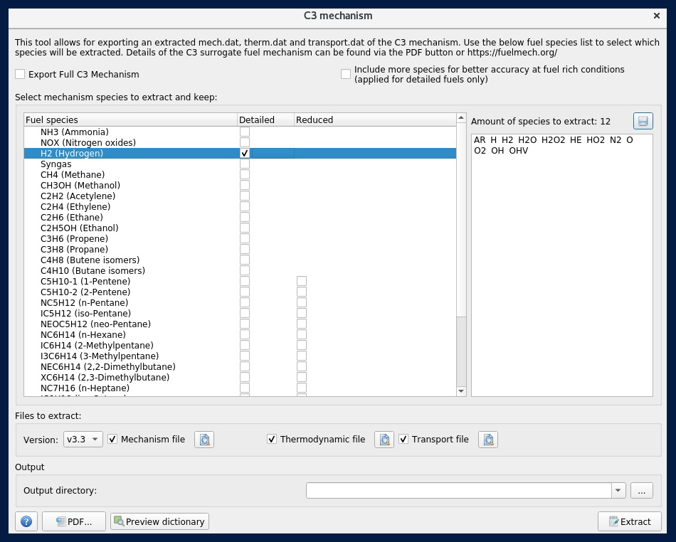
In most cases involving traditional hydrocarbon fuels, your extracted mechanism will have hundreds to thousands of species, which is far too many to use for a 3D CFD simulation. To ensure computational efficiency while maintaining solution accuracy, you should reduce your mechanism to a manageable size using CONVERGE’s mechanism reduction process.
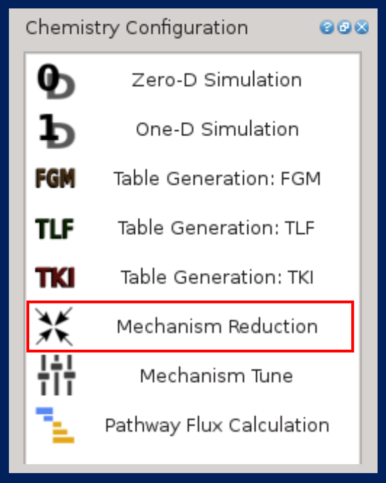
A key component of this process in CONVERGE is the analysis of autoignition, extinction, speciation, and/or laminar flamespeed simulations. Therefore, before you can begin your reduction process, you must consider the specific conditions of your engine/combustor under which these simulations are evaluated. These operating conditions include pressure, unburnt temperature, equivalence ratio, and EGR fractions. For example, if your mechanism is meant to be used for a diesel engine simulation, you must select a pressure range from the start of injection to peak cylinder pressure.
To reduce the number of species, a directed relation graph (DRG) will be constructed and error propagation (DRGEP) can be added for further precision. The DRGEP methodology works to remove species and corresponding reactions within the user-specified error bounds of ignition delay, extinction, speciation, and/or laminar flamespeed. Once the number of species is ~500, sensitivity analysis (SA) can be added to the existing DRGEP methodology for further reduction of species. The optimal resulting mechanism will have calculations that fall within a user-specified range and a reduced number of species, making these mechanisms practical for 3D combustion simulations.
When you have obtained the optimal reduced mechanism, the reaction rates of the most sensitive reactions can be tuned to match specific targets of this mechanism to those of the parent mechanism. Similarly to the reduction process, these targets are speciation, extinction, laminar flamespeed, and/or ignition delay. You can tune your mechanism using CONVERGE’s mechanism tuning tools, such as NLOPT, an open-source library for nonlinear local and global optimization; the MONTE-CARLO method, which uses randomization to solve problems that may be deterministic in principle; or CONGO, CONVERGE’s in-house genetic algorithm optimization tool. These methods focus on the pre-exponential factor, A, or the activation energy in the Arrhenius reaction equation.
After completing these steps, your reduced chemical mechanism is ready to be run in 3D CFD simulations. The flexibility, versatility, and ingenuity of C3 simplifies the process of modeling both traditional and alternative fuels in a variety of applications where combustion is involved. With C3, your days of manually searching through the literature for a specific mechanism are over. Welcome to a new era of ease!
If you would like to help set the direction of future C3 efforts and have access to our mechanisms before they are publicly available, we invite you to join our consortium. To learn more, please contact C3 Director Dr. Kelly Senecal at senecal@fuelmech.org.
Researchers from GM and University of Utah used FLOW-3D WELD to understand mixing of dissimilar metals through laser keyhole welding. They looked at the effect of laser power and scan speed on the mixing concentration of copper and aluminum as it relates to recoil pressure and Marangoni convection. They compared simulations with experimental results and found good agreement between material concentrations at cut cross sections within the samples.
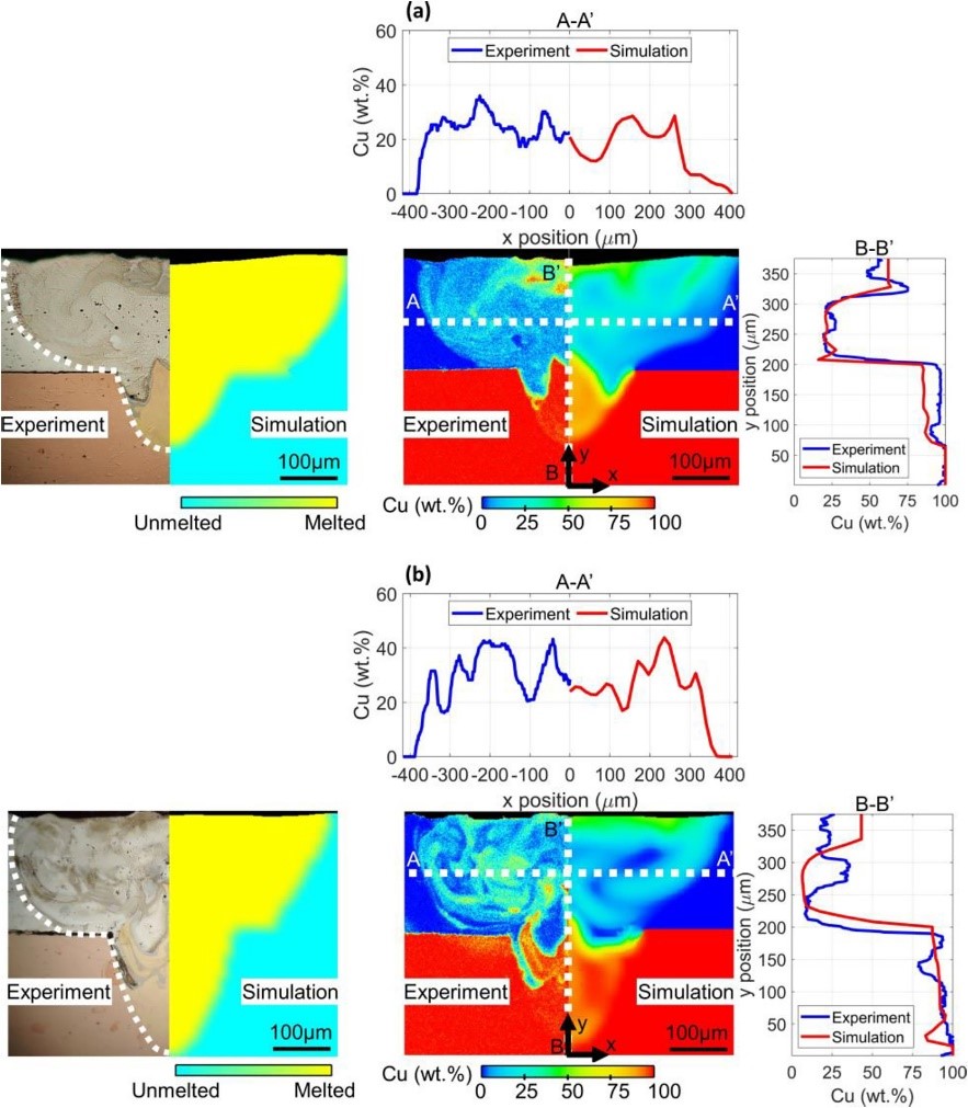
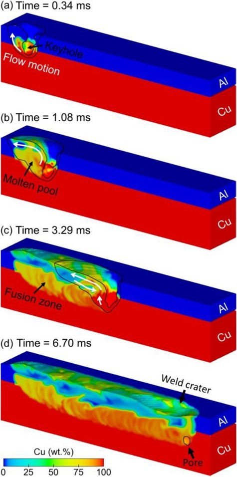
Reference: Wenkang Huang, Hongliang Wang, Teresa Rinker, Wenda Tan, Investigation of metal mixing in laser keyhole welding of dissimilar metals, Materials & Design, Volume 195, (2020). https://doi.org/10.1016/j.matdes.2020.109056
Researchers at GM Global R&D and Southern Methodist University used FLOW-3D WELD to understand how process parameters and laser beam inclination influenced the seam quality in laser brazing of galvanized steels. Due to the low boiling point of zinc, the early vaporization caused spatter and other defects. Using simulation, the researchers predicted the positions of the Zinc evaporation front and the wetting front, and by subsequently controlling the beam angle of inclination, the entrainment of the Zinc vapor within the melt pool was mitigated. This resulted in a stable process and a good braze quality.

Reference: Masoud Mohammadpour, Baixuan Yang, Hui-Ping Wang, John Forrest, Michael Poss, Blair Carlson, Radovan Kovacevica, Influence of laser beam inclination angle on galvanized steel laser braze quality, Optics and Laser Technology, 129; 106303, 2020. doi.org/10.1016/j.optlastec.
How is porosity formed during keyholing? This was the question that researchers from TU Denmark answered using FLOW-3D WELD. As the substrate melts under the application of a laser beam, the recoil pressure due to phase change depresses the melt pool. The co-existence of a downward flow due to recoil pressure and the additional laser energy absorption due to laser reflections causes a runaway effect, transitioning the melt pool into a keyhole. Eventually, due to the varying temperature along the keyhole wall, surface tension forces cause the wall to pinch off and result in voids that can get trapped by the advancing solidification front, resulting in porosity. This can be seen in the video below.
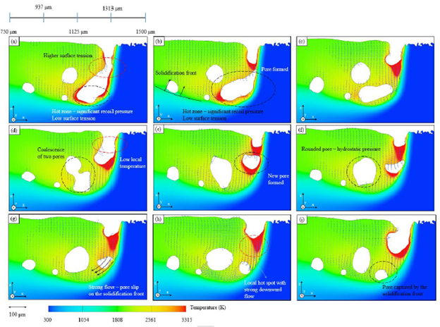
Reference: Mohamad Bayat, Aditi Thanki, Sankhya Mohanty, Ann Witvrouw, Shoufeng Yang, Jesper Thorborg, Niels Skat Tieldje, and Jesper Henri Hattel, Keyhole-induced porosities in Laser-based Powder Bed Fusion (L-PBF) of Ti6Al4V: High-fidelity modelling and experimental validation, Additive Manufacturing, Vol. 30, 2019. doi.org/10.1016/j.addma.2019.100835


Graphcore has used a range of technologies from Mentor, a Siemens business, to successfully design and verify its latest M2000 platform based on the Graphcore Colossus™ GC200 Intelligence Processing Unit (IPU) processor.
Simcenter™ FLOEFD™ software, a CAD-embedded computational fluid dynamics (CFD) tool is part of the Simcenter portfolio of simulation and test solutions that enables companies optimize designs and deliver innovations faster and with greater confidence. Simcenter FLOEFD helps engineers simulate fluid flow and thermal problems quickly and accurately within their preferred CAD environment including NX, Solid Edge, Creo or CATIA V5. With this release, Simcenter FLOEFD helps users create thermal models of electronics packages easily and quickly. Watch this short video to learn how.
Simcenter™ FLOEFD™ software, a CAD-embedded computational fluid dynamics (CFD) tool is part of the Simcenter portfolio of simulation and test solutions that enables companies optimize designs and deliver innovations faster and with greater confidence. Simcenter FLOEFD helps engineers simulate fluid flow and thermal problems quickly and accurately within their preferred CAD environment including NX, Solid Edge, Creo or CATIA V5. With this release, Simcenter FLOEFD allows users to add a component into a direct current (DC) electro-thermal calculation by the given component’s electrical resistance. The corresponding Joule heat is calculated and applied to the body as a heat source. Watch this short video to learn how.
Simcenter™ FLOEFD™ software, a CAD-embedded computational fluid dynamics (CFD) tool is part of the Simcenter portfolio of simulation and test solutions that enables companies optimize designs and deliver innovations faster and with greater confidence. Simcenter FLOEFD helps engineers simulate fluid flow and thermal problems quickly and accurately within their preferred CAD environment including NX, Solid Edge, Creo or CATIA V5. With this release, the software features a new battery model extraction capability that can be used to extract the Equivalent Circuit Model (ECM) input parameters from experimental data. This enables you to get to the required input parameters faster and easier. Watch this short video to learn how.
Simcenter™ FLOEFD™ software, a CAD-embedded computational fluid dynamics (CFD) tool is part of the Simcenter portfolio of simulation and test solutions that enables companies optimize designs and deliver innovations faster and with greater confidence. Simcenter FLOEFD helps engineers simulate fluid flow and thermal problems quickly and accurately within their preferred CAD environment including NX, Solid Edge, Creo or CATIA V5. With this release, Simcenter FLOEFD allows users to create a compact Reduced Order Model (ROM) that solves at a faster rate, while still maintaining a high level of accuracy. Watch this short video to learn how.
High semiconductor temperatures may lead to component degradation and ultimately failure. Proper semiconductor thermal management is key for design safety, reliability and mission critical applications.
A common question from Tecplot 360 users centers around the hardware that they should buy to achieve the best performance. The answer is invariably, it depends. That said, we’ll try to demystify how Tecplot 360 utilizes your hardware so you can make an informed decision in your hardware purchase.
Let’s have a look at each of the major hardware components on your machine and show some test results that illustrate the benefits of improved hardware.
Our test data is an OVERFLOW simulation of a wind turbine. The data consists of 5,863 zones, totaling 263,075,016 elements and the file size is 20.9GB. For our test we:
The test was performed using 1, 2, 4, 8, 16, and 32 CPU-cores, with the data on a local HDD (spinning hard drive) and local SSD (solid state disk). Limiting the number of CPU cores was done using Tecplot 360’s ––max-available-processors command line option.
Data was cleared from the disk cache between runs using RamMap.
Advice: Buy the fastest disk you can afford.
In order to generate any plot in Tecplot 360, you need to load data from a disk. Some plots require more data to be loaded off disk than others. Some file formats are also more efficient than others – particularly file formats that summarize the contents of the file in a single header portion at the top or bottom of the file – Tecplot’s SZPLT is a good example of a highly efficient file format.
We found that the SSD was 61% faster than the HDD when using all 32 CPU-cores for this post-processing task.
All this said – if your data are on a remote server (network drive, cloud storage, HPC, etc…), you’ll want to ensure you have a fast disk on the remote resource and a fast network connection.
With Tecplot 360 the SZPLT file format coupled with the SZL Server could help here. With FieldView you could run in client-server mode.
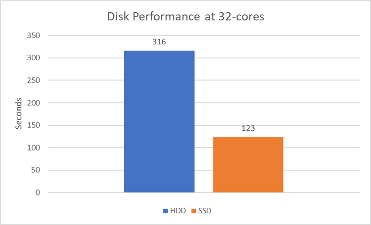
Advice: Buy the fastest CPU, with the most cores, that you can afford. But realize that performance is not always linear with the number of cores.
Most of Tecplot 360’s data compute algorithms are multi-threaded – meaning they’ll use all available CPU-cores during the computation. These include (but are not limited to): Calculation of new variables, slices, iso-surfaces, streamtraces, and interpolations. The performance of these algorithms improves linearly with the number of CPU-cores available.
You’ll also notice that the overall performance improvement is not linear with the number of CPU-cores. This is because loading data off disk becomes a dominant operation, and the slope is bound to asymptote to the disk read speed.
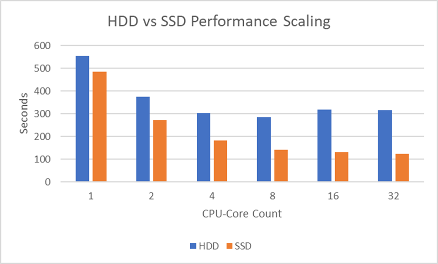
You might notice that the HDD performance actually got worse beyond 8 CPU-cores. We believe this is because the HDD on this machine was just too slow to keep up with 16 and 32 concurrent threads requesting data.
It’s important to note that with data on the SSD the performance improved all the way to 32 CPU-cores. Further reinforcing the earlier advice – buy the fastest disk you can afford.
Advice: Buy as much RAM as you need, but no more.
You might be thinking: “Thanks for nothing – really, how much RAM do I need?”
Well, that’s something you’re going to have to figure out for yourself. The more data Tecplot 360 needs to load to create your plot, the more RAM you’re going to need. Computed iso-surfaces can also be a large consumer of RAM – such as the iso-surface computed in this test case.
If you have transient data, you may want enough RAM to post-process a couple time steps simultaneously – as Tecplot 360 may start loading a new timestep before unloading data from an earlier timestep.
The amount of RAM required is going to be different depending on your file format, cell types, and the post-processing activities you’re doing. For example:
When testing the amount of RAM used by Tecplot 360, make sure to set the Load On Demand strategy to Minimize Memory Use (available under Options>Performance).
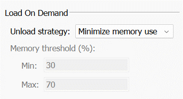
This will give you an understanding of the minimum amount of RAM required to accomplish your task. When set to Auto Unload (the default), Tecplot 360 will maintain more data in RAM, which improves performance. The amount of data Tecplot 360 holds in RAM is dictated by the Memory threshold (%) field, seen in the image above. So you – the user – have control over how much RAM Tecplot 360 is allowed to consume.
Advice: Most modern graphics cards are adequate, even Intel integrated graphics provide reasonable performance. Just make sure you have up to date graphics drivers. If you have an Nvidia graphics card, favor the “Studio” drivers over the “Game Ready” drivers. The “Studio” drivers are typically more stable and offer better performance for the types of plots produced by Tecplot 360.
Many people ask specifically what type of graphics card they should purchase. This is, interestingly, the least important hardware component (at least for most of the plots our users make). Most of the post-processing pipeline is dominated by the disk and CPU, so the time spent rendering the scene is a small percentage of the total.
That said – there are some scenes that will stress your graphics card more than others. Examples are:
Note that Tecplot 360’s interactive graphics performance currently (2023) suffers on Apple Silicon (M1 & M2 chips). The Tecplot development team is actively investigating solutions.
As with most things in life, striking a balance is important. You can spend a huge amount of money on CPUs and RAM, but if you have a slow disk or slow network connection, you’re going to be limited in how fast your post-processor can load the data into memory.
So, evaluate your post-processing activities to try to understand which pieces of hardware may be your bottleneck.
For example, if you:
And again – make sure you have enough RAM for your workflow.
The post What Computer Hardware Should I Buy for Tecplot 360? appeared first on Tecplot Website.
Three years after our merger began, we can report that the combined FieldView and Tecplot team is stronger than ever. Customers continue to receive the highest quality support and new product releases and we have built a solid foundation that will allow us to continue contributing to our customers’ successes long into the future.
This month we have taken another step by merging the FieldView website into www.tecplot.com. Our social media outreach will also be combined. Stay up to date with news and announcements by subscribing and following us on social media.
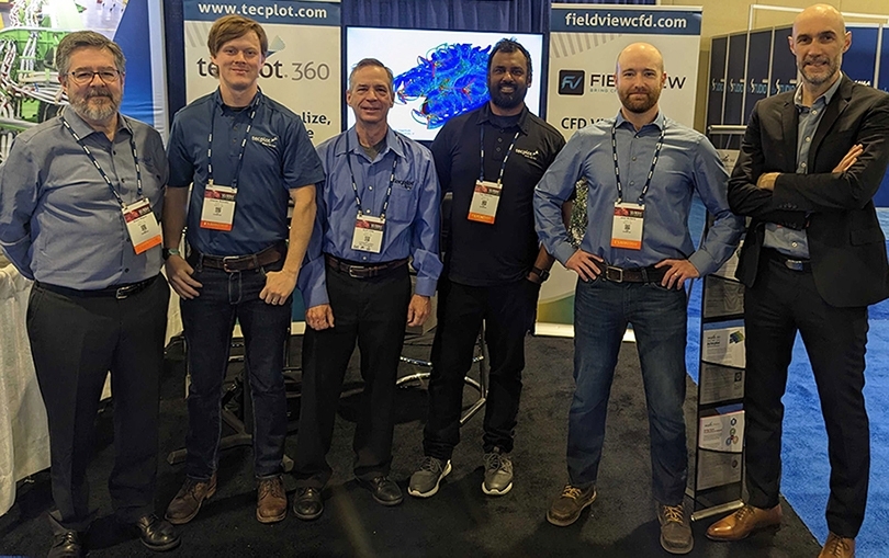
Members of Tecplot 360 & FieldView teams exhibit together at AIAA SciTech 2023. From left to right: Shane Wagner, Charles Schnake, Scott Imlay, Raja Olimuthu, Jared McGarry and Yves-Marie Lefebvre. Not shown are Scott Fowler and Brandon Markham.
It’s been a pleasure seeing two groups that were once competitors come together as a team, learn from each other and really enjoy working together.
– Yves-Marie Lefebvre, Tecplot CTO & FieldView Product Manager.
Our customers have seen some of the benefits of our merger in the form of streamlined services from the common Customer Portal, simplified licensing, and license renewals. Sharing expertise and assets across teams has already led to the faster implementation of modules such as licensing and CFD data loaders. By sharing our development resources, we’ve been able to invest more in new technology, which will soon translate to increased performance and new features for all products.
Many of the improvements are internal to our organization but will have lasting benefits for our customers. Using common development tools and infrastructure will enable us to be as efficient as possible to ensure we can put more of our energy into improving the products. And with the backing of the larger organization, we have a firm foundation to look long term at what our customers will need in years to come.
We want to thank our customers and partners for their support and continued investment as we endeavor to create better tools that empower engineers and scientists to discover, analyze and understand information in complex data, and effectively communicate their results.
The post FieldView joins Tecplot.com – Merger Update appeared first on Tecplot Website.
One of the most memorable parts of my finite-elements class in graduate school was a comparison of linear elements and higher-order elements for the structural analysis of a dam. As I remember, they were able to duplicate the results obtained with 34 linear elements by using a SINGLE high-order element. This made a big impression on me, but the skills I learned at that time remained largely unused until recently.
You see, my Ph.D. research and later work was using finite-volume CFD codes to solve the steady-state viscous flow. For steady flows, there didn’t seem to be much advantage to using higher than 2nd or 3rd order accuracy.
This has changed recently as the analysis of unsteady vortical flows have become more common. The use of higher-order (greater than second order) computational fluid dynamics (CFD) methods is increasing. Popular government and academic CFD codes such as FUN3D, KESTREL, and SU2 have released, or are planning to release, versions that include higher-order methods. This is because higher-order accurate methods offer the potential for better accuracy and stability, especially for unsteady flows. This trend is likely to continue.
Commercial visual analysis codes are not yet providing full support for higher-order solutions. The CFD 2030 vision states
“…higher-order methods will likely increase in utilization during this time frame, although currently the ability to visualize results from higher order simulations is highly inadequate. Thus, software and hardware methods to handle data input/output (I/O), memory, and storage for these simulations (including higher-order methods) on emerging HPC systems must improve. Likewise, effective CFD visualization software algorithms and innovative information presentation (e.g., virtual reality) are also lacking.”
The isosurface algorithm described in this paper is the first step toward improving higher-order element visualization in the commercial visualization code Tecplot 360.
Higher-order methods can be based on either finite-difference methods or finite-element methods. While some popular codes use higher-order finite-difference methods (OVERFLOW, for example), this paper will focus on higher-order finite-element techniques. Specifically, we will present a memory-efficient recursive subdivision algorithm for visualizing the isosurface of higher-order element solutions.
In previous papers we demonstrated this technique for quadratic tetrahedral, hexahedral, pyramid, and prism elements with Lagrangian polynomial basis functions. In this paper Optimized Implementation of Recursive Sub-Division Technique for Higher-Order Finite-Element Isosurface and Streamline Visualization we discuss the integration of these techniques into the engine of the commercial visualization code Tecplot 360 and discuss speed optimizations. We also discuss the extension of the recursive subdivision algorithm to cubic tetrahedral and pyramid elements, and quartic tetrahedral elements. Finally, we discuss the extension of the recursive subdivision algorithm to the computation of streamlines.
Click an image to view the slideshow
[See image gallery at www.tecplot.com]The post Faster Visualization of Higher-Order Finite-Element Data appeared first on Tecplot Website.
In this release, we are very excited to offer “Batch-Pack” licensing for the first time. A Batch-Pack license enables a single user access to multiple concurrent batch instances of our Python API (PyTecplot) while consuming only a single license seat. This option will reduce license contention and allow for faster turnaround times by running jobs in parallel across multiple nodes of an HPC. All at a substantially lower cost than buying additional license seats.
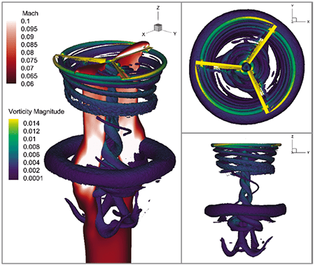
Data courtesy of ZJ Wang, University of Kansas, visualization by Tecplot.
Get a Free Trial Update Your Software
The post Webinar: Tecplot 360 2022 R2 appeared first on Tecplot Website.
Call 1.800.763.7005 or 425.653.1200
Email info@tecplot.com
Batch-mode is a term nearly as old as computers themselves. Despite its age, however, it is representative of a concept that is as relevant today as it ever was, perhaps even more so: headless (scripted, programmatic, automated, etc.) execution of instructions. Lots of engineering is done interactively, of course, but oftentimes the task is a known quantity and there is a ton of efficiency to be gained by automating the computational elements. That efficiency is realized ten times over when batch-mode meets parallelization – and that’s why we thought it was high-time we offered a batch-mode licensing model for Tecplot 360’s Python API, PyTecplot. We call them “batch-packs.”
Tecplot 360 batch-packs work by enabling users to run multiple concurrent instances of our Python API (PyTecplot) while consuming only a single license seat. It’s an optional upgrade that any customer can add to their license for a fee. The benefit? The fee for a batch-pack is substantially lower than buying an equivalent number of license seats – which makes it easier to justify outfitting your engineers with the software access they need to reach peak efficiency.
Here is a handy little diagram we drew to help explain it better:
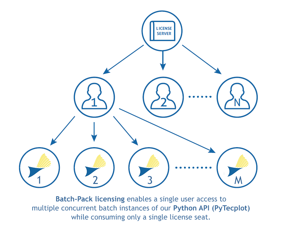
Each network license allows ‘n’ seats. Traditionally, each instance of PyTecplot consumes 1 seat. Prior to the 2022 R2 release of Tecplot 360 EX, licenses only operated using the paradigm illustrated in the first two rows of the diagram above (that is, a user could check out up to ‘n’ seats, or ‘n’ users could check out a single seat). Now customers can elect to purchase batch-packs, which will enable each seat to provide a single user with access to ‘m’ instances of PyTecplot, as shown in the bottom row of the figure.
In addition to a cost reduction (vs. purchasing an equivalent number of network seats), batch-pack licensees will enjoy:
We’re excited to offer this new option and hope that our customers can make the most of it.
The post Introducing 360 “Batch-Packs” appeared first on Tecplot Website.
If you care about how you present your data and how people perceive your results, stop reading and watch this talk by Kristen Thyng on YouTube. Seriously, I’ll wait, I’ve got the time.
Which colormap you choose, and which data values are assigned to each color can be vitally important to how you (or your clients) interpret the data being presented. To illustrate the importance of this, consider the image below.
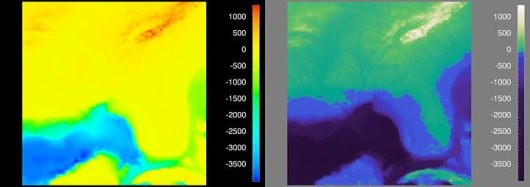
Figure 1. Visualization of the Southeast United States. [4]
Before I explain what a perceptually uniform colormap is, let’s start with everyone’s favorite: the rainbow colormap. We all love the rainbow colormap because it’s pretty and is recognizable. Everyone knows “ROY G BIV” so we think of this color progression as intuitive, but in reality (for scalar values) it’s anything but.
Consider the image below, which represents the “Estimated fraction of precipitation lost to evapotranspiration”. This image makes it appear that there’s a very distinct difference in the scalar value right down the center of the United States. Is there really a sudden change in the values right in the middle of the Great Plains? No – this is an artifact of the colormap, which is misleading you!
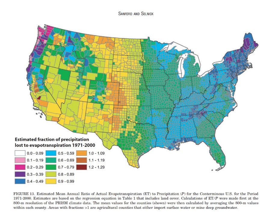
Figure 2. This plot illustrates how the rainbow colormap is misleading, giving the perception that there is a distinct different in the middle of the US, when in fact the values are more continuous. [2]
So let’s dive a little deeper into the rainbow colormap and how it compares to perceptually uniform (or perceptually linear) colormaps.
Consider the six images below, what are we looking at? If you were to only look at the top three images, you might get the impression that the scalar value has non-linear changes – while this value (radius) is actually changing linearly. If presented with the rainbow colormap, you’d be forgiven if you didn’t guess that the object is a cone, colored by radius.
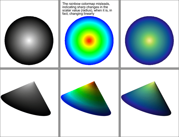
Figure 3. An example of how the rainbow colormap imparts information that does not actually exist in the data.
So why does the rainbow colormap mislead? It’s because the color values are not perceptually uniform. In this image you can see how the perceptual changes in the colormap vary from one end to the other. The gray scale and “cmocean – haline” colormaps shown here are perceptually uniform, while the rainbow colormap adds information that doesn’t actually exist.

Figure 4. Visualization of the perceptual changes of three colormaps. [5]
Well, that depends. Tecplot 360 and FieldView are typically used to represent scalar data, so Sequential and Diverging colormaps will probably get used the most – but there are others we will discuss as well.
Sequential colormaps are ideal for scalar values in which there’s a continuous range of values. Think pressure, temperature, and velocity magnitude. Here we’re using the ‘cmocean – thermal’ colormap in Tecplot 360 to represent fluid temperature in a Barracuda Virtual Reactor simulation of a cyclone separator.
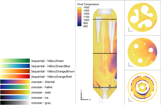
Diverging colormaps are a great option when you want to highlight a change in values. Think ratios, where the values span from -1 to 1, it can help to highlight the value at zero.
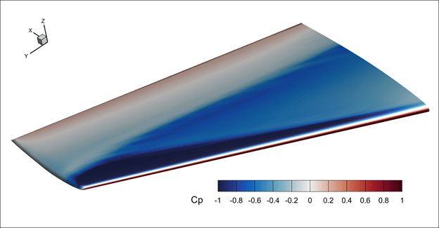
The diverging colormap is also useful for “delta plots” – In the plot below, the bottom frame is showing a delta between the current time step and the time average. Using a diverging colormap, it’s easy to identify where the delta changes from negative to positive.
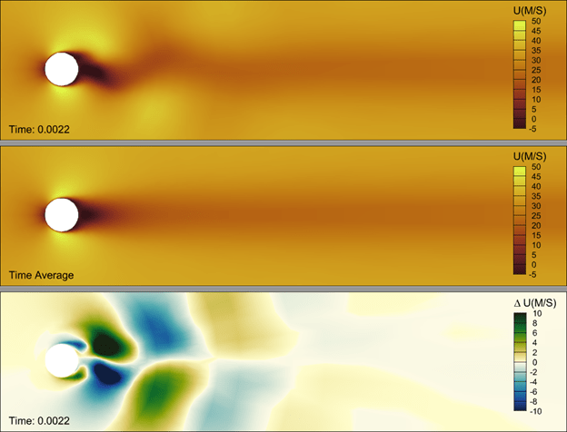
If you have discrete data that represent things like material properties – say “rock, sand, water, oil”, these data can be represented using integer values and a qualitative colormap. This type of colormap will do good job in supplying distinct colors for each value. An example of this, from a CONVERGE simulation, can be seen below. Instructions to create this plot can be found in our blog, Creating a Materials Legend in Tecplot 360.
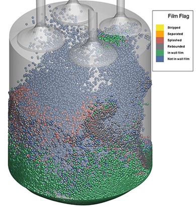
Perhaps infrequently used, but still important to point out is the “phase” colormap. This is particularly useful for values which are cyclic – such as a theta value used to represent wind direction in this FVCOM simulation result. If we were to use a simple sequential colormap (inset plot below) you would observe what appears to be a large gradient where the wind direction is 360o vs. 0o. Logically these are the same value and using the “cmocean – phase” colormap allows you communicate the continuous nature of the data.
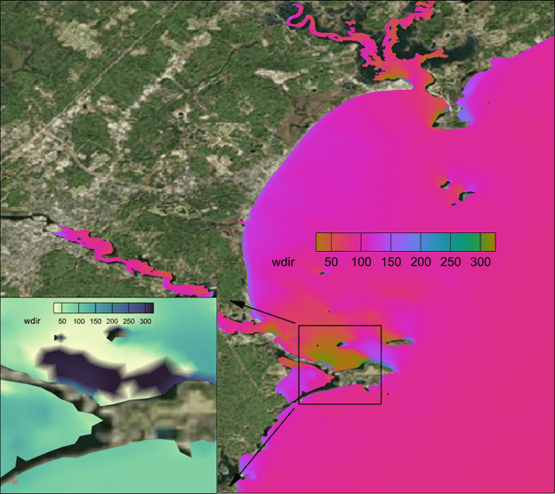
There are times when you want to force a break in a continuous colormap. In the image below, the colormap is continuous from green to white ![]() but we want to ensure that values at or below zero are represented as blue – to indicate water. In Tecplot 360 this can be done using the “Override band colors” option, in which we override the first color band to be blue. This makes the plot more realistic and therefore easier to interpret.
but we want to ensure that values at or below zero are represented as blue – to indicate water. In Tecplot 360 this can be done using the “Override band colors” option, in which we override the first color band to be blue. This makes the plot more realistic and therefore easier to interpret.
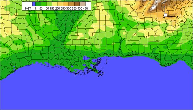
The post Colormap in Tecplot 360 appeared first on Tecplot Website.

Ansys has announced that it will acquire Zemax, maker of high-performance optical imaging system simulation solutions. The terms of the deal were not announced, but it is expected to close in the fourth quarter of 2021.
Zemax’s OpticStudio is often mentioned when users talk about designing optical, lighting, or laser systems. Ansys says that the addition of Zemax will enable Ansys to offer a “comprehensive solution for simulating the behavior of light in complex, innovative products … from the microscale with the Ansys Lumerical photonics products, to the imaging of the physical world with Zemax, to human vision perception with Ansys Speos [acquired with Optis]”.
This feels a lot like what we’re seeing in other forms of CAE, for example, when we simulate materials from nano-scale all the way to fully-produced-sheet-of-plastic-scale. There is something to be learned at each point, and simulating them all leads, ultimately, to a more fit-for-purpose end result.
Ansys is acquiring Zemax from its current owner, EQT Private Equity. EQT’s announcement of the sale says that “[w]ith the support of EQT, Zemax expanded its management team and focused on broadening the Company’s product portfolio through substantial R&D investment focused on the fastest growing segments in the optics space. Zemax also revamped its go-to-market sales approach and successfully transitioned the business model toward recurring subscription revenue”. EQT had acquired Zemax in 2018 from Arlington Capital Partners, a private equity firm, which had acquired Zemax in 2015. Why does this matter? Because the path each company takes is different — and it’s sometimes not a straight line.
Ansys says the transaction is not expected to have a material impact on its 2021 financial results.

Last year Sandvik acquired CGTech, makers of Vericut. I, like many people, thought “well, that’s interesting” and moved on. Then in July, Sandvik announced it was snapping up the holding company for Cimatron, GibbsCAM (both acquired by Battery Ventures from 3D Systems), and SigmaTEK (acquired by Battery Ventures in 2018). Then, last week, Sandvik said it was adding Mastercam to that list … It’s clearly time to dig a little deeper into Sandvik and why it’s doing this.
First, a little background on Sandvik. Sandvik operates in three main spheres: rocks, machining, and materials. For the rocks part of the business, the company makes mining/rock extraction and rock processing (crushing, screening, and the like) solutions. Very cool stuff but not relevant to the CAM discussion.
The materials part of the business develops and sells industrial materials; Sandvik is in the process of spinning out this business. Also interesting but …
The machining part of the business is where things get more relevant to us. Sandvik Machining & Manufacturing Solutions (SMM) has been supplying cutting tools and inserts for many years, via brands like Sandvik, SECO, Miranda, Walter, and Dormer Pramet, and sees a lot of opportunity in streamlining the processes around the use of specific tools and machines. Light weighting and sustainability efforts in end-industries are driving interest in new materials and more complex components, as well as tighter integration between design and manufacturing operations. That digitalization across an enterprise’s areas of business, Sandvik thinks, plays into its strengths.
According to info from the company’s 2020 Capital Markets Day, rocks and materials are steady but slow revenue growers. The company had set a modest 5% revenue growth target but had consistently been delivering closer to 3% — what to do? Like many others, the focus shifted to (1) software and (2) growth by acquisition. Buying CAM companies ticked both of those boxes, bringing repeatable, profitable growth. In an area the company already had some experience in.
Back to digitalization. If we think of a manufacturer as having (in-house or with partners) a design function, which sends the concept on to production preparation, then to machining, and, finally, to verification/quality control, Sandvik wants to expand outwards from machining to that entire world. Sandvik wants to help customers optimize the selection of tools, the machining strategy, and the verification and quality workflow.
The Manufacturing Solutions subdivision within SMM was created last year to go after this opportunity. It’s got 3 areas of focus: automating the manufacturing process, industrializing additive manufacturing, and expanding the use of metrology to real-time decision making.
The CGTech acquisition last year was the first step in realizing this vision. Vericut is prized for its ability to work with any CAM, machine tool, and cutting tool for NC code simulation, verification, optimization, and programming. CGTech is a long-time supplier of Vericut software to Sandvik’s Coromant production units, so the companies knew one another well. Vericut helps Sandvik close that digitalization/optimization loop — and, of course, gives it access to the many CAM users out there who do not use Coromant.
But verification is only one part of the overall loop, and in some senses, the last. CAM, on the other hand, is the first (after design). Sanvik saw CAM as “the most important market to enter due to attractive growth rates – and its proximity to Sandvik Manufacturing and Machining Solutions’ core business.” Adding Cimatron, GibbsCAM, SigmaTEK, and Mastercam gets Sandvik that much closer to offering clients a set of solutions to digitize their complete workflows.
And it makes business sense to add CAM to the bigger offering:
To head off one question: As of last week’s public statements, anyway, Sandvik has no interest in getting into CAD, preferring to leave that battlefield to others, and continue on its path of openness and neutrality.
And because some of you asked: there is some overlap in these acquisitions, but remarkably little, considering how established these companies all are. GibbsCAM is mostly used for production milling and turning; Cimatron is used in mold and die — and with a big presence in automotive, where Sandvik already has a significant interest; and SigmaNEST is for sheet metal fabrication and material requisitioning.
One interesting (to me, anyway) observation: 3D Systems sold Gibbs and Cimatron to Battery in November 2020. Why didn’t Sandvik snap it up then? Why wait until July 2021? A few possible reasons: Sandvik CEO Stefan Widing has been upfront about his company’s relative lack of efficiency in finding/closing/incorporating acquisitions; perhaps it was simply not ready to do a deal of this type and size eight months earlier. Another possible reason: One presumes 3D Systems “cleaned up” Cimatron and GibbsCAM before the sale (meaning, separating business systems and financials from the parent, figuring out HR, etc.) but perhaps there was more to be done, and Sandvik didn’t want to take that on. And, finally, maybe the real prize here for Sandvik was SigmaNEST, which Battery Ventures had acquired in 2018, and Cimatron and GibbsCAM simply became part of the deal. We may never know.
This whole thing is fascinating. A company out of left field, acquiring these premium PLMish assets. Spending major cash (although we don’t know how much because of non-disclosures between buyer and sellers) for a major market presence.
No one has ever asked me about a CAM roll-up, yet I’m constantly asked about how an acquirer could create another Ansys. Perhaps that was the wrong question, and it should have been about CAM all along. It’s possible that the window for another company to duplicate what Sandvik is doing may be closing since there are few assets left to acquire.
Sandvik’s CAM acquisitions haven’t closed yet, but assuming they do, there’s a strong fit between CAM and Sandvik’s other manufacturing-focused business areas. It’s more software, with its happy margins. And, finally, it lets Sandvik address the entire workflow from just after component design to machining and on to verification. Mr. Widing says that Sandvik first innovated in hardware, then in service – and now, in software to optimize the component part manufacturing process. These are where gains will come, he says, in maximizing productivity and tool longevity. Further out, he sees, measuring every part to see how the process can be further optimized. It’s a sound investment in the evolution of both Sandvik and manufacturing.
We all love a good reinvention story, and how Sandvik executes on this vision will, of course, determine if the reinvention was successful. And, of course, there’s always the potential for more news of this sort …
I missed this last month — Sandvik also acquired Cambrio, which is the combined brand for what we might know better as GibbsCAM (milling, turning), Cimatron (mold and die), and SigmaNEST (nesting, obvs). These three were spun out of 3D Systems last year, acquired by Battery Ventures — and now sold on to Sandvik.
This was announced in July, and the acquisition is expected to close in the second half of 2021 — we’ll find out on Friday if it already has.
At that time. Sandvik said its strategic aim is to “provide customers with software solutions enabling automation of the full component manufacturing value chain – from design and planning to preparation, production and verification … By acquiring Cambrio, Sandvik will establish an important position in the CAM market that includes both toolmaking and general-purpose machining. This will complement the existing customer offering in Sandvik Manufacturing Solutions”.
Cambrio has around 375 employees and in 2020, had revenue of about $68 million.
If we do a bit of math, Cambrio’s $68 million + CNC Software’s $60 million + CGTech’s (that’s Vericut’s maker) of $54 million add up to $182 million in acquired CAM revenue. Not bad.
More on Friday.
CNC Software and its Mastercam have been a mainstay among CAM providers for decades, marketing its solutions as independent, focused on the workgroup and individual. That is about to change: Sandvik, which bought CGTech late last year, has announced that it will acquire CNC Software to build out its CAM offerings.
According to Sandvik’s announcement, CNC Software brings a “world-class CAM brand in the Mastercam software suite with an installed base of around 270,000 licenses/users, the largest in the industry, as well as a strong market reseller network and well-established partnerships with leading machine makers and tooling companies”.
We were taken by surprise by the CGTech deal — but shouldn’t be by the Mastercam acquisition. Stefan Widing, Sandvik’s CEO explains it this way: “[Acquiring Mastercam] is in line with our strategic focus to grow in the digital manufacturing space, with special attention on industrial software close to component manufacturing. The acquisition of CNC Software and the Mastercam portfolio, in combination with our existing offerings and extensive manufacturing capabilities, will make Sandvik a leader in the overall CAM market, measured in installed base. CAM plays a vital role in the digital manufacturing process, enabling new and innovative solutions in automated design for manufacturing.” The announcement goes on to say, “CNC Software has a strong market position in CAM, and particularly for small and medium-sized manufacturing enterprises (SME’s), something that will support Sandvik’s strategic ambitions to develop solutions to automate the manufacturing value chain for SME’s – and deliver competitive point solutions for large original equipment manufacturers (OEM’s).”
Sandvik says that CNC Software has 220 employees, with revenue of $60 million in 2020, and a “historical annual growth rate of approximately 10 percent and is expected to outperform the estimated market growth of 7 percent”.
No purchase price was disclosed, but the deal is expected to close during the fourth quarter.
Sandvik is holding a call about this on Friday — more updates then, if warranted.

Bentley continues to grow its deep expertise in various AEC disciplines — most recently, expanding its focus in underground resource mapping and analysis. This diversity serves it well; read on.
In Q2,
Unlike AspenTech, Bentley’s revenue growth is speeding up (total revenue up 21% in Q2, including a wee bit from Seequent, and up 17% for the first six months of 2021). Why the difference? IMHO, because Bentley has a much broader base, selling into many more end industries as well as to road/bridge/water/wastewater infrastructure projects that keep going, Covid or not. CEO Greg Bentley told investors that some parts of the business are back to —or even better than— pre-pandemic levels, but not yet all. He said that the company continues to struggle in industrial and resources capital expenditure projects, and therefore in the geographies (theMiddle East and Southeast Asia) that are the most dependent on this sector. This is balanced against continued success in new accounts and the company’s reinvigorated selling to small and medium enterprises via its Virtuosity subsidiary — and in a resurgence in the overall commercial/facilities sector. In general, it appears that sales to contractors such as architects and engineers lag behind those to owners and operators of commercial facilities —makes sense as many new projects are still on pause until pandemic-related effects settle down.
One unusual comment from Bentley’s earnings call that we’re going to listen for on others: The government of China is asking companies to explain why they are not using locally-grown software solutions; it appears to be offering preferential tax treatment for buyers of local software. As Greg Bentley told investors, “[d]uring the year to date, we have experienced a rash of unanticipated subscription cancellations within the mid-sized accounts in China that have for years subscribed to our China-specific enterprise program … Because we don’t think there are product issues, we will try to reinstate these accounts through E365 programs, where we can maintain continuous visibility as to their usage and engagement”. So, to recap: the government is using taxation to prefer one set of vendors over another, and all Bentley can do (really) is try to bring these accounts back and then monitor them constantly to keep on top of emerging issues. FWIW, in the pre-pandemic filings for Bentley’s IPO, “greater China, which we define as the Peoples’ Republic of China, Hong Kong and Taiwan … has become one of our largest (among our top five) and fastest-growing regions as measured by revenue, contributing just over 5% of our 2019 revenues”. Something to watch.
The company updated its financial outlook for 2021 to include the recent Seequent acquisition and this moderate level of economic uncertainty. Bentley might actually join the billion-dollar club on a pro forma basis — as if the acquisition of Seequent had occurred at the beginning of 2021. On a reported basis, the company sees total revenue between $945 million and $960 million, or an increase of around 18%, including Seequent. Excluding Seequent, Bentley sees organic revenue growth of 10% to 11%.
Much more here, on Bentley’s investor website.
We still have to hear from Autodesk, but there’s been a lot of AECish earnings news over the last few weeks. This post starts a modest series as we try to catch up on those results.
AspenTech reported results for its fiscal fourth quarter, 2021 last week. Total revenue of $198 million in DQ4, down 2% from a year ago. License revenue was $145 million, down 3%; maintenance revenue was $46 million, basically flat when compared to a year earlier, and services and other revenue was $7 million, up 9%.
For the year, total revenue was up 19% to $709 million, license revenue was up 28%, maintenance was up 4% and services and other revenue was down 18%.
Looking ahead, CEO Antonio Pietri said that he is “optimistic about the long-term opportunity for AspenTech. The need for our customers to operate their assets safely, sustainably, reliably and profitably has never been greater … We are confident in our ability to return to double-digit annual spend growth over time as economic conditions and industry budgets normalize.” The company sees fiscal 2022 total revenue of $702 million to $737 million, which is up just $10 million from final 2021 at the midpoint.
Why the slowdown in FQ4 from earlier in the year? And why the modest guidance for fiscal 2022? One word: Covid. And the uncertainty it creates among AspenTech’s customers when it comes to spending precious cash. AspenTech expects its visibility to improve when new budgets are set in the calendar fourth quarter. By then, AspenTech hopes, its customers will have a clearer view of reopening, consumer spending, and the timing of an eventual recovery.
Lots more detail here on AspenTech’s investor website.
Next up, Bentley. Yup. Alphabetical order.
There is an interesting new trend in using Computational Fluid Dynamics (CFD). Until recently CFD simulation was focused on existing and future things, think flying cars. Now we see CFD being applied to simulate fluid flow in the distant past, think fossils.
CFD shows Ediacaran dinner party featured plenty to eat and adequate sanitation
Let's first address the elephant in the room - it's been a while since the last Caedium release. The multi-substance infrastructure for the Conjugate Heat Transfer (CHT) capability was a much larger effort than I anticipated and consumed a lot of resources. This lead to the relative quiet you may have noticed on our website. However, with the new foundation laid and solid we can look forward to a bright future.
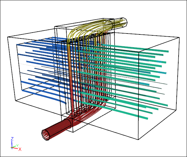 Conjugate Heat Transfer Through a Water-Air Radiator
Simulation shows separate air and water streamline paths colored by temperature
It turns out that Computational Fluid Dynamics (CFD) has a key role to play in determining the behavior of long extinct creatures. In a previous, post we described a CFD study of parvancorina, and now Pernille Troelsen at Liverpool John Moore University is using CFD for insights into how long-necked plesiosaurs might have swum and hunted.
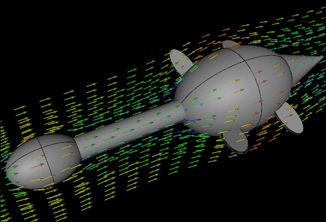 CFD Water Flow Simulation over an Idealized Plesiosaur: Streamline VectorsIllustration only, not part of the study
Fossilized imprints of Parvancorina from over 500 million years ago have puzzled paleontologists for decades. What makes it difficult to infer their behavior is that Parvancorina have none of the familiar features we might expect of animals, e.g., limbs, mouth. In an attempt to shed some light on how Parvancorina might have interacted with their environment researchers have enlisted the help of Computational Fluid Dynamics (CFD).
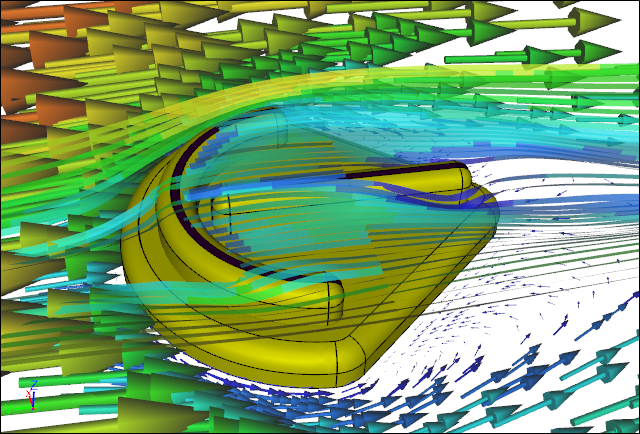 CFD Water Flow Simulation over a Parvancorina: Forward directionIllustration only, not part of the study
One of nature's smallest aerodynamic specialists - insects - have provided a clue to more efficient and robust wind turbine design.
 Dragonfly: Yellow-winged DarterLicense: CC BY-SA 2.5, André Karwath
The recent attempt to break the 2 hour marathon came very close at 2:00:24, with various aids that would be deemed illegal under current IAAF rules. The bold and obvious aerodynamic aid appeared to be a Tesla fitted with an oversized digital clock leading the runners by a few meters.
2 Hour Marathon Attempt
In this post, I’ll give a simple example of how to create curves in blockMesh. For this example, we’ll look at the following basic setup:

As you can see, we’ll be simulating the flow over a bump defined by the curve:
First, let’s look at the basic blockMeshDict for this blocking layout WITHOUT any curves defined:
/*--------------------------------*- C++ -*----------------------------------*\
  =========                 |
  \\      /  F ield         | OpenFOAM: The Open Source CFD Toolbox
   \\    /   O peration     | Website:  https://openfoam.org
    \\  /    A nd           | Version:  6
     \\/     M anipulation  |
\*---------------------------------------------------------------------------*/
FoamFile
{
    version     2.0;
    format      ascii;
    class       dictionary;
    object      blockMeshDict;
}

// * * * * * * * * * * * * * * * * * * * * * * * * * * * * * * * * * * * * * //

convertToMeters 1;

vertices
(
    (-1 0 0)    // 0
    (0 0 0)     // 1
    (1 0 0)     // 2
    (2 0 0)     // 3
    (-1 2 0)    // 4
    (0 2 0)     // 5
    (1 2 0)     // 6
    (2 2 0)     // 7

    (-1 0 1)    // 8
    (0 0 1)     // 9
    (1 0 1)     // 10
    (2 0 1)     // 11
    (-1 2 1)    // 12
    (0 2 1)     // 13
    (1 2 1)     // 14
    (2 2 1)     // 15
);

blocks
(
    hex (0 1 5 4 8 9 13 12) (20 100 1) simpleGrading (0.1 10 1)
    hex (1 2 6 5 9 10 14 13) (80 100 1) simpleGrading (1 10 1)
    hex (2 3 7 6 10 11 15 14) (20 100 1) simpleGrading (10 10 1)
);

edges
(
);

boundary
(
    inlet
    {
        type patch;
        faces
        (
            (0 8 12 4)
        );
    }
    outlet
    {
        type patch;
        faces
        (
            (3 7 15 11)
        );
    }
    lowerWall
    {
        type wall;
        faces
        (
            (0 1 9 8)
            (1 2 10 9)
            (2 3 11 10)
        );
    }
    upperWall
    {
        type patch;
        faces
        (
            (4 12 13 5)
            (5 13 14 6)
            (6 14 15 7)
        );
    }
    frontAndBack
    {
        type empty;
        faces
        (
            (8 9 13 12)
            (9 10 14 13)
            (10 11 15 14)
            (1 0 4 5)
            (2 1 5 6)
            (3 2 6 7)
        );
    }
);

// ************************************************************************* //
This blockMeshDict produces the following grid:

It is best practice in my opinion to first make your blockMesh without any edges. This lets you see if there are any major errors resulting from the block topology itself. From the results above, we can see we’re ready to move on!
So now we need to define the curve. In blockMesh, curves are added using the edges sub-dictionary. This is a simple sub dictionary that is just a list of interpolation points:
edges
(
        polyLine 1 2
        (
                (0	0       0)
                (0.1	0.0309016994    0)
                (0.2	0.0587785252    0)
                (0.3	0.0809016994    0)
                (0.4	0.0951056516    0)
                (0.5	0.1     0)
                (0.6	0.0951056516    0)
                (0.7	0.0809016994    0)
                (0.8	0.0587785252    0)
                (0.9	0.0309016994    0)
                (1	0       0)
        )

        polyLine 9 10
        (
                (0	0       1)
                (0.1	0.0309016994    1)
                (0.2	0.0587785252    1)
                (0.3	0.0809016994    1)
                (0.4	0.0951056516    1)
                (0.5	0.1     1)
                (0.6	0.0951056516    1)
                (0.7	0.0809016994    1)
                (0.8	0.0587785252    1)
                (0.9	0.0309016994    1)
                (1	0       1)
        )
);
The sub-dictionary above is just a list of points on the curve 

The following mesh is produced:

Hopefully this simple example will help some people looking to incorporate curved edges into their blockMeshing!
Cheers.
This offering is not approved or endorsed by OpenCFD Limited, producer and distributor of the OpenFOAM software via http://www.openfoam.com, and owner of theOPENFOAM® andOpenCFD® trademarks.
Experimentally visualizing high-speed flow was a serious challenge for decades. Before the advent of modern laser diagnostics and velocimetry, the only real techniques for visualizing high speed flow fields were the optical techniques of Schlieren and Shadowgraph.
Today, Schlieren and Shadowgraph remain an extremely popular means to visualize high-speed flows. In particular, Schlieren and Shadowgraph allow us to visualize complex flow phenomena such as shockwaves, expansion waves, slip lines, and shear layers very effectively.
In CFD there are many reasons to recreate these types of images. First, they look awesome. Second, if you are doing a study comparing to experiments, occasionally the only full-field data you have could be experimental images in the form of Schlieren and Shadowgraph.
Without going into detail about Schlieren and Shadowgraph themselves, primarily you just need to understand that Schlieren and Shadowgraph represent visualizations of the first and second derivatives of the flow field refractive index (which is directly related to density).
In Schlieren, a knife-edge is used to selectively cut off light that has been refracted. As a result you get a visualization of the first derivative of the refractive index in the direction normal to the knife edge. So for example, if an experiment used a horizontal knife edge, you would see the vertical derivative of the refractive index, and hence the density.
For Shadowgraph, no knife edge is used, and the images are a visualization of the second derivative of the refractive index. Unlike the Schlieren images, shadowgraph has no direction and shows you the laplacian of the refractive index field (or density field).
In this post, I’ll use a simple case I did previously (https://curiosityfluids.com/2016/03/28/mach-1-5-flow-over-23-degree-wedge-rhocentralfoam/) as an example and produce some synthetic Schlieren and Shadowgraph images using the data.
Well as you might expect, from the introduction, we simply do this by visualizing the gradients of the density field.
In ParaView the necessary tool for this is:
Gradient of Unstructured DataSet:

Once you’ve selected this, we then need to set the properties so that we are going to operate on the density field:

To do this, simply set the “Scalar Array” to the density field (rho), and change the name of the result Array name to SyntheticSchlieren. Now you should see something like this:

There are a few problems with the above image (1) Schlieren images are directional and this is a magnitude (2) Schlieren and Shadowgraph images are black and white. So if you really want your Schlieren images to look like the real thing, you should change to black and white. ALTHOUGH, Cold and Hot, Black-Body radiation, and Rainbow Desatured all look pretty amazing.
To fix these, you should only visualize one component of the Synthetic Schlieren array at a time, and you should visualize using the X-ray color preset:

The results look pretty realistic:


The process of computing the shadowgraph field is very similar. However, recall that shadowgraph visualizes the Laplacian of the density field. BUT THERE IS NO LAPLACIAN CALCULATOR IN PARAVIEW!?! Haha no big deal. Just remember the basic vector calculus identity:
Therefore, in order for us to get the Shadowgraph image, we just need to take the Divergence of the Synthetic Schlieren vector field!
To do this, we just have to use the Gradient of Unstructured DataSet tool again:

This time, Deselect “Compute Gradient” and the select “Compute Divergence” and change the Divergence array name to Shadowgraph.
Visualized in black and white, we get a very realistic looking synthetic Shadowgraph image:

Now this is an important question, but a simple one to answer. And the answer is…. not much. Physically, we know exactly what these mean, these are: Schlieren is the gradient of the density field in one direction and Shadowgraph is the laplacian of the density field. But what you need to remember is that both Schlieren and Shadowgraph are qualitative images. The position of the knife edge, brightness of the light etc. all affect how a real experimental Schlieren or Shadowgraph image will look.
This means, very often, in order to get the synthetic Schlieren to closely match an experiment, you will likely have to change the scale of your synthetic images. In the end though, you can end up with extremely realistic and accurate synthetic Schlieren images.
Hopefully this post will be helpful to some of you out there. Cheers!
Sutherland’s equation is a useful model for the temperature dependence of the viscosity of gases. I give a few details about it in this post: https://curiosityfluids.com/2019/02/15/sutherlands-law/
The law given by:
It is also often simplified (as it is in OpenFOAM) to:
In order to use these equations, obviously, you need to know the coefficients. Here, I’m going to show you how you can simply create your own Sutherland coefficients using least-squares fitting Python 3.
So why would you do this? Basically, there are two main reasons for this. First, if you are not using air, the Sutherland coefficients can be hard to find. If you happen to find them, they can be hard to reference, and you may not know how accurate they are. So creating your own Sutherland coefficients makes a ton of sense from an academic point of view. In your thesis or paper, you can say that you created them yourself, and not only that you can give an exact number for the error in the temperature range you are investigating.
So let’s say we are looking for a viscosity model of Nitrogen N2 – and we can’t find the coefficients anywhere – or for the second reason above, you’ve decided its best to create your own.
By far the simplest way to achieve this is using Python and the Scipy.optimize package.
Step 1: Get Data
The first step is to find some well known, and easily cited, source for viscosity data. I usually use the NIST webbook (
https://webbook.nist.gov/), but occasionally the temperatures there aren’t high enough. So you could also pull the data out of a publication somewhere. Here I’ll use the following data from NIST:
| Temparature (K) | Viscosity (Pa.s) |
| 200 |
0.000012924 |
| 400 | 0.000022217 |
| 600 | 0.000029602 |
| 800 | 0.000035932 |
| 1000 | 0.000041597 |
| 1200 | 0.000046812 |
| 1400 | 0.000051704 |
| 1600 | 0.000056357 |
| 1800 | 0.000060829 |
| 2000 | 0.000065162 |
This data is the dynamics viscosity of nitrogen N2 pulled from the NIST database for 0.101 MPa. (Note that in these ranges viscosity should be only temperature dependent).
Step 2: Use python to fit the data
If you are unfamiliar with Python, this may seem a little foreign to you, but python is extremely simple.
First, we need to load the necessary packages (here, we’ll load numpy, scipy.optimize, and matplotlib):
import numpy as np
import matplotlib.pyplot as plt
from scipy.optimize import curve_fit
Now we define the sutherland function:
def sutherland(T, As, Ts):
    return As*T**(3/2)/(Ts+T)
Next we input the data:
T=[200,
400,
600,
800,
1000,
1200,
1400,
1600,
1800,
2000]

mu=[0.000012924,
0.000022217,
0.000029602,
0.000035932,
0.000041597,
0.000046812,
0.000051704,
0.000056357,
0.000060829,
0.000065162]
Then we fit the data using the curve_fit function from scipy.optimize. This function uses a least squares minimization to solve for the unknown coefficients. The output variable popt is an array that contains our desired variables As and Ts.
popt = curve_fit(sutherland, T, mu)
As=popt[0]
Ts=popt[1]
Now we can just output our data to the screen and plot the results if we so wish:
print('As = '+str(popt[0])+'\n')
print('Ts = '+str(popt[1])+'\n')

xplot=np.linspace(200,2000,100)
yplot=sutherland(xplot,As,Ts)

plt.plot(T,mu,'ok',xplot,yplot,'-r')
plt.xlabel('Temperature (K)')
plt.ylabel('Dynamic Viscosity (Pa.s)')
plt.legend(['NIST Data', 'Sutherland'])
plt.show()
Overall the entire code looks like this:
import numpy as np
import matplotlib.pyplot as plt
from scipy.optimize import curve_fit

def sutherland(T, As, Ts):
    return As*T**(3/2)/(Ts+T)

T=[200, 400, 600,
800,
1000,
1200,
1400,
1600,
1800,
2000]

mu=[0.000012924,
0.000022217,
0.000029602,
0.000035932,
0.000041597,
0.000046812,
0.000051704,
0.000056357,
0.000060829,
0.000065162]

popt, pcov = curve_fit(sutherland, T, mu)
As=popt[0]
Ts=popt[1]
print('As = '+str(popt[0])+'\n')
print('Ts = '+str(popt[1])+'\n')

xplot=np.linspace(200,2000,100)
yplot=sutherland(xplot,As,Ts)

plt.plot(T,mu,'ok',xplot,yplot,'-r')
plt.xlabel('Temperature (K)')
plt.ylabel('Dynamic Viscosity (Pa.s)')
plt.legend(['NIST Data', 'Sutherland'])
plt.show()
And the results for nitrogen gas in this range are As=1.55902E-6, and Ts=168.766 K. Now we have our own coefficients that we can quantify the error on and use in our academic research! Wahoo!

In this post, we looked at how we can simply use a database of viscosity-temperature data and use the python package scipy to solve for our unknown Sutherland viscosity coefficients. This NIST database was used to grab some data, and the data was then loaded into Python and curve-fit using scipy.optimize curve_fit function.
This task could also easily be accomplished using the Matlab curve-fitting toolbox, or perhaps in excel. However, I have not had good success using the excel solver to solve for unknown coefficients.
The most common complaint I hear, and the most common problem I observe with OpenFOAM is its supposed “steep learning curve”. I would argue however, that for those who want to practice CFD effectively, the learning curve is equally as steep as any other software.
There is a distinction that should be made between “user friendliness” and the learning curve required to do good CFD.
While I concede that other commercial programs have better basic user friendliness (a nice graphical interface, drop down menus, point and click options etc), it is equally as likely (if not more likely) that you will get bad results in those programs as with OpenFOAM. In fact, to some extent, the high user friendliness of commercial software can encourage a level of ignorance that can be dangerous. Additionally, once you are comfortable operating in the OpenFOAM world, the possibilities become endless and things like code modification, and bash and python scripting can make OpenFOAM worklows EXTREMELY efficient and powerful.
Anyway, here are a few tips to more easily tackle the OpenFOAM learning curve:
(1) Understand CFD
This may seem obvious… but its not to some. Troubleshooting bad simulation results or unstable simulations that crash is impossible if you don’t have at least a basic understanding of what is happening under the hood. My favorite books on CFD are:
(a) The Finite Volume Method in Computational Fluid Dynamics: An Advanced Introduction with OpenFOAM® and Matlab by
F. Moukalled, L. Mangani, and M. Darwish
(b) An introduction to computational fluid dynamics – the finite volume method – by H K Versteeg and W Malalasekera
(c) Computational fluid dynamics – the basics with applications – By John D. Anderson
(2) Understand fluid dynamics
Again, this may seem obvious and not very insightful. But if you are going to assess the quality of your results, and understand and appreciate the limitations of the various assumptions you are making – you need to understand fluid dynamics. In particular, you should familiarize yourself with the fundamentals of turbulence, and turbulence modeling.
(3) Avoid building cases from scratch
Whenever I start a new case, I find the tutorial case that most closely matches what I am trying to accomplish. This greatly speeds things up. It will take you a super long time to set up any case from scratch – and you’ll probably make a bunch of mistakes, forget key variable entries etc. The OpenFOAM developers have done a lot of work setting up the tutorial cases for you, so use them!
As you continue to work in OpenFOAM on different projects, you should be compiling a library of your own templates based on previous work.
(4) Using Ubuntu makes things much easier
This is strictly my opinion. But I have found this to be true. Yes its true that Ubuntu has its own learning curve, but I have found that OpenFOAM works seamlessly in the Ubuntu or any Ubuntu-like linux environment. OpenFOAM now has Windows flavors using docker and the like- but I can’t really speak to how well they work – mostly because I’ve never bothered. Once you unlock the power of Linux – the only reason to use Windows is for Microsoft Office (I guess unless you’re a gamer – and even then more and more games are now on Linux). Not only that- but the VAST majority of forums and troubleshooting associated with OpenFOAM you’ll find on the internet are from Ubuntu users.
I much prefer to use Ubuntu with a virtual Windows environment inside it. My current office setup is my primary desktop running Ubuntu – plus a windows VirtualBox, plus a laptop running windows that I use for traditional windows type stuff. Dual booting is another option, but seamlessly moving between the environments is easier.
(5) If you’re struggling, simplify
Unless you know exactly what you are doing, you probably shouldn’t dive into the most complicated version of whatever you are trying to solve/study. It is best to start simple, and layer the complexity on top. This way, when something goes wrong, it is much easier to figure out where the problem is coming from.
(6) Familiarize yourself with the cfd-online forum
If you are having trouble, the cfd-online forum is super helpful. Most likely, someone else is has had the same problem you have. If not, the people there are extremely helpful and overall the forum is an extremely positive environment for working out the kinks with your simulations.
(7) The results from checkMesh matter
If you run checkMesh and your mesh fails – fix your mesh. This is important. Especially if you are not planning on familiarizing yourself with the available numerical schemes in OpenFOAM, you should at least have a beautiful mesh. In particular, if your mesh is highly non-orthogonal, you will have serious problems. If you insist on using a bad mesh, you will probably need to manipulate the numerical schemes. A great source for how schemes should be manipulated based on mesh non-orthogonality is:
http://www.wolfdynamics.com/wiki/OFtipsandtricks.pdf
(8) CFL Number Matters
If you are running a transient case, the Courant-Freidrechs-Lewis (CFL) number matters… a lot. Not just for accuracy (if you are trying to capture a transient event) but for stability. If your time-step is too large you are going to have problems. There is a solid mathematical basis for this stability criteria for advection-diffusion problems. Additionally the Navier-Stokes equations are very non-linear and the complexity of the problem and the quality of your grid etc can make the simulation even less stable. When I have a transient simulation crash, if I know my mesh is OK, I decrease the timestep by a factor of 2. More often than not, this solves the problem.
For large time stepping, you can add outer loops to solvers based on the pimple algorithm, but you may end up losing important transient information. Excellent explanation of how to do this is given in the book by T. Holzmann:
https://holzmann-cfd.de/publications/mathematics-numerics-derivations-and-openfoam
For the record, this points falls into point (1) of Understanding CFD.
(9) Work through the OpenFOAM Wiki “3 Week” Series
If you are starting OpenFOAM for the first time, it is worth it to work through an organized program of learning. One such example (and there are others) is the “3 Weeks Series” on the OpenFOAM wiki:
https://wiki.openfoam.com/%223_weeks%22_series
If you are a graduate student, and have no job to do other than learn OpenFOAM, it will not take 3 weeks. This touches on all the necessary points you need to get started.
(10) OpenFOAM is not a second-tier software – it is top tier
I know some people who have started out with the attitude from the get-go that they should be using a different software. They think somehow Open-Source means that it is not good. This is a pretty silly attitude. Many top researchers around the world are now using OpenFOAM or some other open source package. The number of OpenFOAM citations has grown every year consistently (
https://www.linkedin.com/feed/update/urn:li:groupPost:1920608-6518408864084299776/?commentUrn=urn%3Ali%3Acomment%3A%28groupPost%3A1920608-6518408864084299776%2C6518932944235610112%29&replyUrn=urn%3Ali%3Acomment%3A%28groupPost%3A1920608-6518408864084299776%2C6518956058403172352%29).
In my opinion, the only place where mainstream commercial CFD packages will persist is in industry labs where cost is no concern, and changing software is more trouble than its worth. OpenFOAM has been widely benchmarked, and widely validated from fundamental flows to hypersonics (see any of my 17 publications using it for this). If your results aren’t good, you are probably doing something wrong. If you have the attitude that you would rather be using something else, and are bitter that your supervisor wants you to use OpenFOAM, when something goes wrong you will immediately think there is something wrong with the program… which is silly – and you may quit.
(11) Meshing… Ugh Meshing
For the record, meshing is an art in any software. But meshing is the only area where I will concede any limitation in OpenFOAM. HOWEVER, as I have outlined in my previous post (https://curiosityfluids.com/2019/02/14/high-level-overview-of-meshing-for-openfoam/) most things can be accomplished in OpenFOAM, and there are enough third party meshing programs out there that you should have no problem.
Basically, if you are starting out in CFD or OpenFOAM, you need to put in time. If you are expecting to be able to just sit down and produce magnificent results, you will be disappointed. You might quit. And frankly, thats a pretty stupid attitude. However, if you accept that CFD and fluid dynamics in general are massive fields under constant development, and are willing to get up to speed, there are few limits to what you can accomplish.
Please take the time! If you want to do CFD, learning OpenFOAM is worth it. Seriously worth it.
This offering is notapproved or endorsed by OpenCFD Limited, producer and distributorof the OpenFOAM software via http://www.openfoam.com, and owner of theOPENFOAM® andOpenCFD® trade marks.

Here I will present something I’ve been experimenting with regarding a simplified workflow for meshing airfoils in OpenFOAM. If you’re like me, (who knows if you are) I simulate a lot of airfoils. Partly because of my involvement in various UAV projects, partly through consulting projects, and also for testing and benchmarking OpenFOAM.
Because there is so much data out there on airfoils, they are a good way to test your setups and benchmark solver accuracy. But going from an airfoil .dat coordinate file to a mesh can be a bit of pain. Especially if you are starting from scratch.
The two main ways that I have meshed airfoils to date has been:
(a) Mesh it in a C or O grid in blockMesh (I have a few templates kicking around for this
(b) Generate a “ribbon” geometry and mesh it with cfMesh
(c) Or back in the day when I was a PhD student I could use Pointwise – oh how I miss it.
But getting the mesh to look good was always sort of tedious. So I attempted to come up with a python script that takes the airfoil data file, minimal inputs and outputs a blockMeshDict file that you just have to run.
The goals were as follows:
(a) Create a C-Grid domain
(b) be able to specify boundary layer growth rate
(c) be able to set the first layer wall thickness
(e) be mostly automatic (few user inputs)
(f) have good mesh quality – pass all checkMesh tests
(g) Quality is consistent – meaning when I make the mesh finer, the quality stays the same or gets better
(h) be able to do both closed and open trailing edges
(i) be able to handle most airfoils (up to high cambers)
(j) automatically handle hinge and flap deflections
In Rev 1 of this script, I believe I have accomplished (a) thru (g). Presently, it can only hand airfoils with closed trailing edge. Hinge and flap deflections are not possible, and highly cambered airfoils do not give very satisfactory results.
There are existing tools and scripts for automatically meshing airfoils, but I found personally that I wasn’t happy with the results. I also thought this would be a good opportunity to illustrate one of the ways python can be used to interface with OpenFOAM. So please view this as both a potentially useful script, but also something you can dissect to learn how to use python with OpenFOAM. This first version of the script leaves a lot open for improvement, so some may take it and be able to tailor it to their needs!
Hopefully, this is useful to some of you out there!
You can download the script here:
https://github.com/curiosityFluids/curiosityFluidsAirfoilMesher
Here you will also find a template based on the airfoil2D OpenFOAM tutorial.
(1) Copy curiosityFluidsAirfoilMesher.py to the root directory of your simulation case.
(2) Copy your airfoil coordinates in Selig .dat format into the same folder location.
(3) Modify curiosityFluidsAirfoilMesher.py to your desired values. Specifically, make sure that the string variable airfoilFile is referring to the right .dat file
(4) In the terminal run: python3 curiosityFluidsAirfoilMesher.py
(5) If no errors – run blockMesh
PS
You need to run this with python 3, and you need to have numpy installed
The inputs for the script are very simple:
ChordLength: This is simply the airfoil chord length if not equal to 1. The airfoil dat file should have a chordlength of 1. This variable allows you to scale the domain to a different size.
airfoilfile: This is a string with the name of the airfoil dat file. It should be in the same folder as the python script, and both should be in the root folder of your simulation directory. The script writes a blockMeshDict to the system folder.
DomainHeight: This is the height of the domain in multiples of chords.
WakeLength: Length of the wake domain in multiples of chords
firstLayerHeight: This is the height of the first layer. To estimate the requirement for this size, you can use the curiosityFluids y+ calculator
growthRate: Boundary layer growth rate
MaxCellSize: This is the max cell size along the centerline from the leading edge of the airfoil. Some cells will be larger than this depending on the gradings used.
The following inputs are used to improve the quality of the mesh. I have had pretty good results messing around with these to get checkMesh compliant grids.
BLHeight: This is the height of the boundary layer block off of the surfaces of the airfoil
LeadingEdgeGrading: Grading from the 1/4 chord position to the leading edge
TrailingEdgeGrading: Grading from the 1/4 chord position to the trailing edge
inletGradingFactor: This is a grading factor that modifies the the grading along the inlet as a multiple of the leading edge grading and can help improve mesh uniformity
trailingBlockAngle: This is an angle in degrees that expresses the angles of the trailing edge blocks. This can reduce the aspect ratio of the boundary cells at the top and bottom of the domain, but can make other mesh parameters worse.
Inputs:

With the above inputs, the grid looks like this:


Mesh Quality:

These are some pretty good mesh statistics. We can also view them in paraView:


The clark-y has some camber, so I thought it would be a logical next test to the previous symmetric one. The inputs I used are basically the same as the previous airfoil:

With these inputs, the result looks like this:


Mesh Quality:

Visualizing the mesh quality:


Here is an example of a flying with airfoil (tested since the trailing edge is tilted upwards).
Inputs:

Again, these are basically the same as the others. I have found that with these settings, I get pretty consistently good results. When you change the MaxCellSize, firstLayerHeight, and Grading some modification may be required. However, if you just half the maxCell, and half the firstLayerHeight, you “should” get a similar grid quality just much finer.


Grid Quality:

Visualizing the grid quality


Hopefully some of you find this tool useful! I plan to release a Rev 2 soon that will have the ability to handle highly cambered airfoils, and open trailing edges, as well as control surface hinges etc.
The long term goal will be an automatic mesher with an H-grid in the spanwise direction so that the readers of my blog can easily create semi-span wing models extremely quickly!
Comments and bug reporting encouraged!
DISCLAIMER: This script is intended as an educational and productivity tool and starting point. You may use and modify how you wish. But I make no guarantee of its accuracy, reliability, or suitability for any use. This offering is not approved or endorsed by OpenCFD Limited, producer and distributor of the OpenFOAM software via http://www.openfoam.com, and owner of the OPENFOAM® and OpenCFD® trademarks.
Here is a useful little tool for calculating the properties across a normal shock.
If you found this useful, and have the need for more, visit www.stfsol.com. One of STF Solutions specialties is providing our clients with custom software developed for their needs. Ranging from custom CFD codes to simpler targeted codes, scripts, macros and GUIs for a wide range of specific engineering purposes such as pipe sizing, pressure loss calculations, heat transfer calculations, 1D flow transients, optimization and more. Visit STF Solutions at www.stfsol.com for more information!
Disclaimer: This calculator is for educational purposes and is free to use. STF Solutions and curiosityFluids makes no guarantee of the accuracy of the results, or suitability, or outcome for any given purpose.

![\nabla^2\left[\right] = \nabla \cdot \nabla \left[\right]](https://s0.wp.com/latex.php?latex=%5Cnabla%5E2%5Cleft%5B%5Cright%5D++%3D+%5Cnabla+%5Ccdot+%5Cnabla+%5Cleft%5B%5Cright%5D&bg=4c5c68&fg=46494c&s=0&c=20201002)


.jpg)